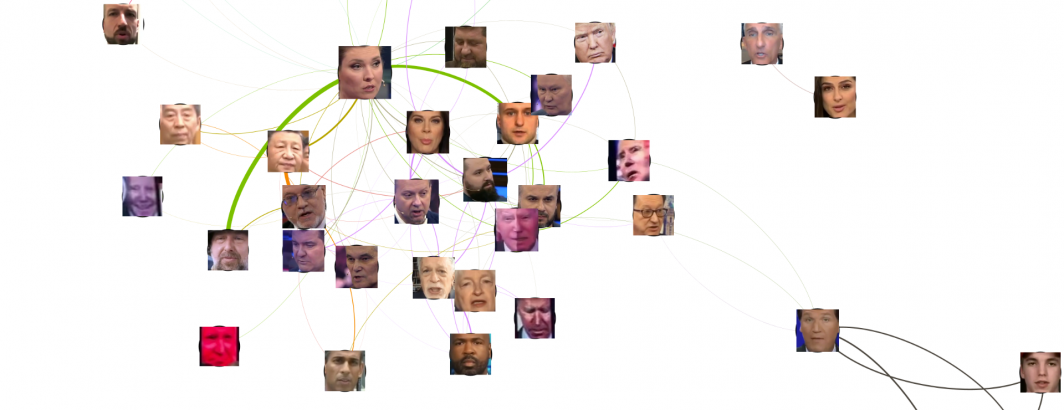
Last week we demonstrated using a simplistic facial extraction and visual clustering pipeline to extract the faces from a single episode of Russian TV News Russia 1's "60 Minutes" and build a co-occurrence graph of who appears alongside of whom. To make the pipeline as easy to use as possible, we used a very simplistic pipeline of an older face extractor that is less accurate than modern tools but extremely fast, coupled with a perceptual hash-based clustering postprocessor to group faces together to track them across frames. The results suggested considerable promise for this analytic approach, but also demonstrated the existential limitations of such a simple pipeline. Today we revisit that exploration using a modern face extraction and clustering pipeline that yields vastly more accurate results.
As before, we are going to analyze an episode of Russia 1's 60 Minutes from March 13th. First we'll download the every-four-seconds preview images from that broadcast from the Visual Explorer:
wget https://storage.googleapis.com/data.gdeltproject.org/gdeltv3/iatv/visualexplorer/RUSSIA1_20230313_083000_60_minut.zip
unzip
Now we're going to download two Python scripts and associated tooling that will extract all of the faces from each image, compute embeddings for each and then cluster the results using DBSCAN.
First, we install the dependencies:
apt-get -y install build-essential
brew install cmake
pip3 install face_recognition
pip3 install imutils
pip3 install argparse
pip3 install scikit-learn
Now we're going to extract all of the faces and encode them as 128-dimension embeddings and store as a pickle. We use the Histogram of Oriented Gradients (HOG) detection method because we are running on a CPU-only system. While the CNN model would likely yield better results this allows us to run without a GPU, though in practice during spot checks we did not identify any obvious failed facial extractions:
wget https://raw.githubusercontent.com/kunalagarwal101/Face-Clustering/master/encode_faces.py
time python3 encode_faces.py --dataset ./RUSSIA1_20230313_083000_60_minut/ --encodings RUSSIA1_20230313_083000_60_minut.encodings.pickle --detection_method "hog"
This runs serially on a single CPU and takes around 20 minutes to extract and encode all of the faces, storing them into a single pickled array. The end result is an array of extracted faces that we need to connect together to determine which faces depict the same person. In other words, we need to cluster all of the faces based on similarity. Since we don't know apriori how many faces to expect, we need a clustering algorithm that does not need a predefined number of clusters, so DBSCAN is used.
We've extensively modified the clustering script that accompanies the above encoding script, including to output the list of matches to STDOUT for use with our downstream graph construction. Save the following Python script to cluster_faces_mod.py:
#MODIFIED FROM https://github.com/kunalagarwal101/Face-Clustering/blob/master/cluster_faces.py

from sklearn.cluster import DBSCAN
from imutils import build_montages
import numpy as np
import argparse
import pickle
import cv2
import shutil
import os
from constants import FACE_DATA_PATH, ENCODINGS_PATH, CLUSTERING_RESULT_PATH

ap = argparse.ArgumentParser()
ap.add_argument("-e", "--encodings", required=True, help="path to serialized db of facial encodings")
ap.add_argument("-j", "--jobs", type=int, default=-1, help="# of parallel jobs to run (-1 will use all CPUs)")
args = vars(ap.parse_args())

print("[INFO] loading encodings...")
data = pickle.loads(open(args["encodings"], "rb").read())
data = np.array(data)
encodings = [d["encoding"] for d in data]

print("[INFO] clustering...")
clt = DBSCAN(metric="euclidean", n_jobs=args["jobs"], eps=0.4)
clt.fit(encodings)

# determine the total number of unique faces found in the dataset
# clt.labels_ contains the label ID for all faces in our dataset (i.e., which cluster each face belongs to).
# To find the unique faces/unique label IDs, used NumPy’s unique function.
# The result is a list of unique labelIDs
labelIDs = np.unique(clt.labels_)

numUniqueFaces = len(np.where(labelIDs > -1)[0])
print("[INFO] # unique faces: {}".format(numUniqueFaces))

for labelID in labelIDs:
	idxs = np.where(clt.labels_ == labelID)[0]
	faces = []
	#print all of the matches
	for i in idxs:
		#write the match
		print("[MATCH] FACEID=\"{}\" IMG=\"{}\"".format(labelID,data[i]["imagePath"]))
		#extract the face so we can use it to build our graph display... extract all so we can find the "best" in post...
		(top, right, bottom, left) = data[i]["loc"]
		image = cv2.imread(data[i]["imagePath"])
		face = image[top:bottom, left:right]
		cv2.imwrite("./FACES/{}-{}.jpg".format(labelID,i), face)
		face = cv2.resize(face, (96, 96))
		faces.append(face)
	montage = build_montages(faces, (96, 96), (10, 20))[0]
	cv2.imwrite("./FACES/montage-{}.jpg".format(labelID), montage)
Note that we modify the DBSCAN invocation to change epsilon to 0.4, which we experimentally found to yield the best results on this dataset – higher values yielded super clusters grouping together different people with highly similar facial structures, while lower values were too sensitive to facial orientation and occlusion.
Then we run:
mkdir FACES
time python3 cluster_faces_mod.py --encodings RUSSIA1_20230313_083000_60_minut.encodings.pickle --jobs -1 > CLUSTER.TXT
To visualize how well the clustering worked, the script above constructs a montage image of thumbnails for each cluster representing a single person. Let's in turn compile all of those together into a single super montage:
mkdir /dev/shm/tmp/; export MAGICK_TEMPORARY_PATH="/dev/shm/tmp/"
time montage FACES/montage*.jpg -mode Concatenate -tile 6x -frame 5 FACES/montage-final.png
You can view the final montage below (NOTE: this is an extremely large image):
The top-left cluster contains all images that DBSCAN was unable to cluster. Adjusting the value of epsilon passed to DBSCAN has a significant impact on recovering some of these images to their correct clusters, but at the cost of degrading some of the clusters' membership. Each of the other clusters represents a group of faces determined to represent a single individual. Note the tremendous range of facial expressions, orientations, occlusions, motion blur, filtering and other differences between the faces within a single cluster and the ability of this pipeline to look across those differences to identify them as belonging to the same individual. In a few cases the differences are so extreme it was unable to correctly group them together – these are typically background images that were displayed on the giant studio television screens behind the presenters and thus are very small, blurry and heavily filtered, making them difficult to cluster, though further refinement of epsilon could likely group these correctly.
Now we run the following PERL script to process the clustering results from above, permute into a final co-occurrence graph (connecting the faces in each frame to the other faces appearing in the same frame and the immediately prior frame – getting at both split-screen and multi-presenter scenes and the back-and-forth camera shots common to 60 Minutes):
#!/usr/bin/perl

#load the CLUSTER file that tells us which extracted faces are the same face...
open(FILE, "./CLUSTER.TXT");
$FACEID = 0;
while(<FILE>) {
    if ($_!~/\[MATCH\]/) { next; };
    ($FACEID, $IMG) = $_=~/FACEID="(.*?)" IMG="(.*?)"/;
    if ($FACEID == -1) { next; }; #skip unclustered...
    ($frame) = $IMG=~/\-(\d\d\d\d\d\d)\.jpg/;
    $FACEIDSBYFRAME{$frame+0}{$FACEID} = 1;
}
close(FILE);

#scan all of the extracted faces to find the largest for each ID... with JPEG compression this is a combination of largest and most complex...
foreach $img (glob("./FACES/*.jpg")) {
    ($id, $seq) = $img=~/(\d+)\-(\d+)\.jpg/;
    $size = (-s $img);
    $img=~s/\.\/FACES\///;
    if ($size > $FACEIMG_SIZE{$id}) { $FACEIMG_SIZE{$id} = $size; $FACEIMG_FILE{$id} = $img; };
}

#now permute the faces to build up the co-occurence graph...
foreach $frame (keys %FACEIDSBYFRAME) {

    my @arr_this = (sort keys %{$FACEIDSBYFRAME{$frame}}); my $arrlen_this = scalar(@arr_this);
    my @arr_prev; if ($frame > 0) { @arr_prev = (sort keys %{$FACEIDSBYFRAME{$frame-1}}); }; my $arrlen_prev = scalar(@arr_prev);
    my $i; my $j;
    for($i=0;$i<$arrlen_this;$i++) {
        #faces that actually co-occurred together in THIS frame...
        for($j=$i+1;$j<$arrlen_this;$j++) {
            $EDGES{"$arr_this[$i],$arr_this[$j]"}+=2;
        }

        #connect to faces from previous frame...
        for($j=0;$j<$arrlen_prev;$j++) {
            if ($arr_this[$i] != $arr_prev[$j]) { $EDGES{"$arr_this[$i],$arr_prev[$j]"}+=1; };
        }
    }
}

#do a pass through the graph and compute the max tie strength to normalize since Gephi wants range 0.0-1.0... also threshold weak ties...
$MAX = 0; $THRESHOLD = 2;
foreach $pair (keys %EDGES) {
    if ($EDGES{$pair} > $MAX) { $MAX = $EDGES{$pair}; };
}
print "MAX = $MAX\n";

#and output the final edges graph...
open(OUT, ">./EDGES.csv");
print OUT "Source,Target,Type,Weight,CocurFrames\n";
$THRESHOLD = 2;
foreach $pair (keys %EDGES) {
    if ($EDGES{$pair} < $THRESHOLD) { next; };
    $weight = sprintf("%0.4f", $EDGES{$pair} / $MAX);
    print OUT "$pair,\"Undirected\",$weight,$EDGES{$pair}\n";
    ($node1, $node2) = split/,/, $pair; $NODES{$node1} = 1; $NODES{$node2} = 1;
}
close(OUT);

#and output the final nodes graph...
open(OUT, ">./NODES.csv");
print OUT "Id,Image\n";
foreach $node (keys %NODES) {
    print OUT "$node,$FACEIMG_FILE{$node}\n";
    $FILENAMES{$FACEIMG_FILE{$node}} = 1;
}
close(OUT);

#and make the filelist of files to copy locally...
open(OUT, ">./FILENAMES.TXT");
foreach $node (keys %FILENAMES) {
    print OUT "$node\n";
}
close(FILE);
This will output three files: a nodes, edges and filenames list. We'll need to extract the list of connected faces to use as our node images in a moment, so this will use the FILENAMES.TXT to extract all of the images into a directory called NODEIMAGES:
mkdir NODEIMAGES
cat FILENAMES.TXT | parallel 'cp FACES/{} NODEIMAGES/'
Now we'll visualize this cooccurrence network using Gephi. Note that we'll specifically need Gephi 0.9.6, not the latest 0.10 release, as the plugin we are going to use is not yet compatible with the latest version. If you don't already have it, install the Image Preview plugin.
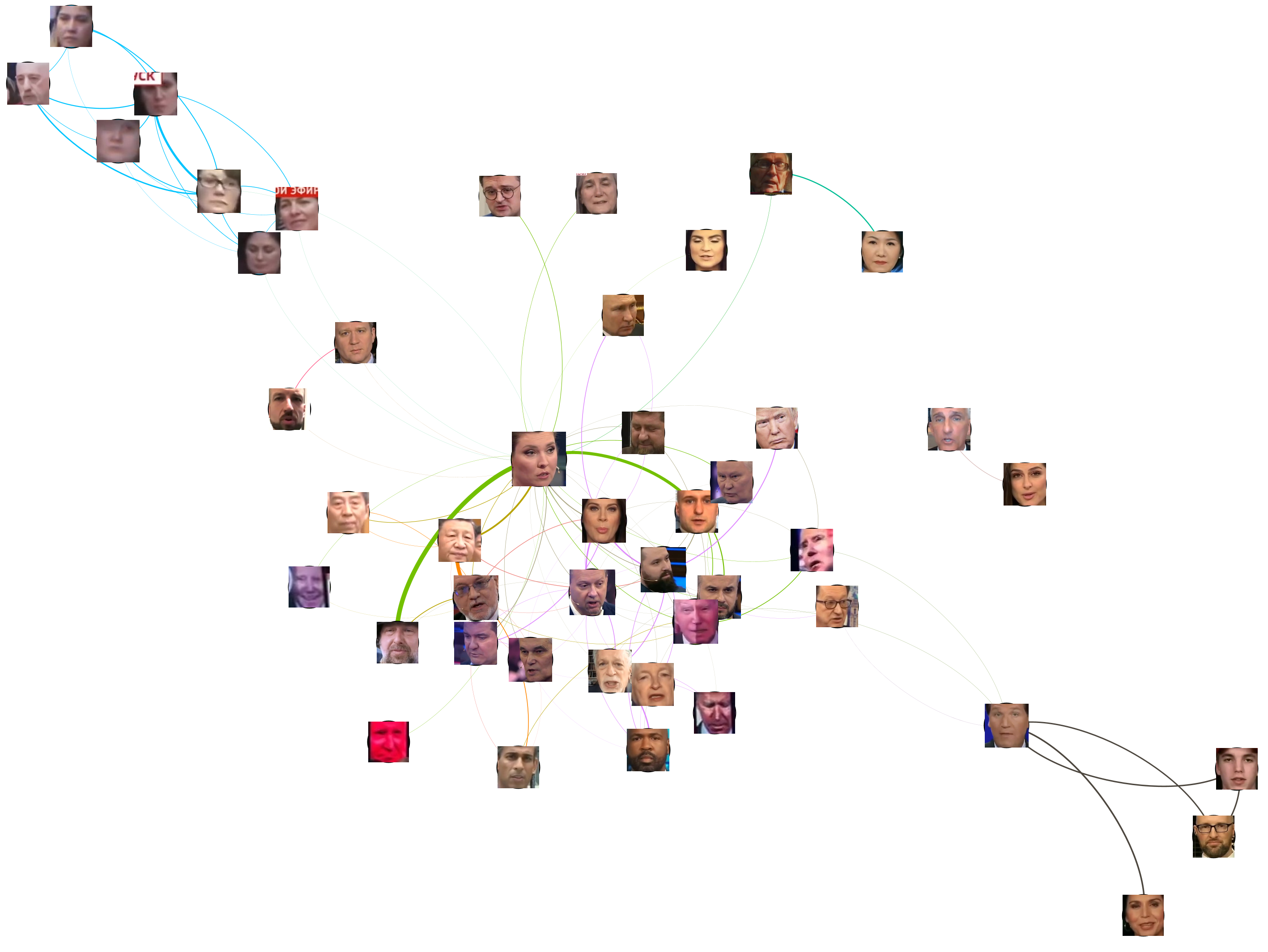
Now open a new workspace and import the Nodes.csv and Edges.csv files into the Data Laboratory. Cluster using the clustering algorithm of your choice. You may also choose to size nodes via PageRank, as we do here. In the Preview window, you may have to enable "Image Nodes" under "Manage renderers". Under Preview Settings at the bottom enable "Render Nodes as Images" and set "Image Path" to the full path where NODEIMAGES is. Then render the graph.
The final visualization can be seen below. Host Olga Skabeyeva appears at the center of the graph, accurately reflecting her central role in each 60 Minutes broadcast. Around her appear the central guests and topics of the evening. The highly interconnected nature of the central cluster around her reflects 60 Minutes' method of storytelling in which a central cast of commentators are interwoven constantly in split-screen and back-and-forth camera shots with the persons being discussed, creating a fast-paced highly interspersed visual sequence of faces that is strikingly different than the sequential studio center-focused and wide shots more typical of American broadcasts. She is most strongly connected to two individuals that she appeared in extended split-screen sequences with. Tucker Carlson, who appeared at the center of the previous visualization due to his fixed head tilt appears here as a weakly connected peripheral cluster strongly tied to his guests, accurately reflecting his small role in this broadcast.
A particularly interesting finding is the array of "Bizarre Biden's" in the central cluster that tend to feature his face snapshotted in particular facial expressions and highly filtered to oversaturate and exaggerate its appearance. These are actually background images displayed on the studio jumbotron-style screens in the background of studio wide shots. They are physically very small and typically capture highly exaggerated poses and expressions, often with post-filtering to oversaturate them, making it extremely difficult for the clustering process to correctly identify them as a single individual. Their presence here at the center of the graph captures their steady background presence in this broadcast as thematic imagery.
We are tremendously excited about the potential of this new approach to understanding the visual storytelling mechanisms of Russian television news – especially how it can help us understand the tightly interwoven nature of its narratives and how these kinds of insights could be coupled with transcriptional analysis to perform multimodal analyses.
This analysis is part of an ongoing collaboration between the Internet Archive and its TV News Archive, the multi-party Media-Data Research Consortium and GDELT.