Who appears alongside whom on television news represents a key editorial decision of what voices to pair. From split-screen displays to the back-and-forth of presenters and guests, understanding co-occurrence patterns on television news offers a powerful lens into the underlying narrative storytelling of a broadcast. What if we could analyze such co-occurrence patterns automatically, generating a network visualization of the faces that appear onscreen in the same frame or subsequent frames over an entire broadcast?
There are two ways cooccurrence can be explored:
- Face Recognition. All of the faces in each frame are connected back to their actual identity using a face recognition tool like Amazon's Rekognition. This is the most accurate and allows for a rich array of downstream analyses such as affiliation analysis (who is being given the opportunity to tell what story), but poses a number of ethical concerns and works only for well-known individuals that appear in Amazon's database.
- Face Clustering. An algorithm is used to extract each human face found in each frame and faces are simply clustered by similarity. No identity is associated with each face – the system literally simply groups faces by how similar they are. This similarity grouping can be performed using facial landmarks (the most accurate and occlusion and orientation-independent (whether the face is looking directly ahead, titled, turned to the side, etc) or simple pixel-level similarity.
Here we are going to use the second option (Face Clustering using pixel similarity grouping). To minimize the computational requirements of the demo, we are going to use two off-the-shelf tools, one to extract all of the faces from each frame as individual JPEG images and the second to group them by pixel-level similarity. A more advanced workflow would use facial landmarks to group faces by similarity to ensure that a titled head or blink of the eyes is correctly handled, but for simplicity's sake we will use pixel-level grouping in this demo.
Here we analyze an episode of Russia 1's 60 Minutes from yesterday.
First we'll download the every-four-seconds preview images from that broadcast from the Visual Explorer:
wget https://storage.googleapis.com/data.gdeltproject.org/gdeltv3/iatv/visualexplorer/RUSSIA1_20230313_083000_60_minut.zip
unzip
Next we'll use an off-the-shelf simple face detection tool called "facedetect" to scan all of the frames, identify sufficiently large and visible human faces and extract each to its own image file:
apt-get -y install imagemagick
apt-get -y install facedetect
mkdir FACES
time find RUSSIA1_20230313_083000_60_minut/ -type f -name '*.jpg' | parallel --eta 'i=0; facedetect {} | while read x y w h; do convert "{}" -crop ${w}x${h}+${x}+${y} "./FACES/{/.}.face.${i}.jpg"; i=$(($i+1)); done'
find FACES/*.jpg | wc -l
This yields 2,334 extracted face images. Note that this tool does not compute facial landmarks – it simply extracts each face as a separate JPEG image. Many of these faces were extracted from the background of frames, making them extremely small and difficult to discern, so we'll remove all faces that are less than 75×75 pixels. You can manually check the dimensions of each extracted face:
time find ./FACES/ -depth -name "*.jpg" -exec file {} \; | sed 's/\(.*jpg\): .* \([0-9]*x[0-9]*\).*/\2 \1/' | awk -F '[x,"./"]' 'int($1) < 75 || int($2) < 75 {print}'
Now we'll move them to a separate directory to exclude them from our analysis:
mkdir TOOSMALL
time find ./FACES/ -depth -name "*.jpg" -exec file {} \; | sed 's/\(.*jpg\): .* \([0-9]*x[0-9]*\).*/\2 \1/' | awk -F '[x,"./"]' 'int($1) < 75 || int($2) < 75 {print}' | cut -d ' ' -f 2 | parallel --eta 'mv {} ./TOOSMALL/{/}'
This leaves us with 1,248 distinct faces.
In essence, at this point we have a directory of JPEG files representing the cropped faces that facedetect found in each frame. But, how do we determine that a face from one frame is the same as a face from another frame? As noted earlier, a production workflow would use a face detection system that extracts the full suite of facial landmarks and compares them across extracted faces to cluster faces regardless of how the face is oriented (directly ahead, tilted, turned to the side, etc), occlusion, eye blink, etc. Instead, our face detection tool above simply extracts faces as JPEG images, so we will use a trivial similarity metric: pixel similarity.
The off-the-shelf tool "findimagedupes" is ideally suited for this task: given a directory of images it computes a perceptual fingerprint for each image, optionally storing it in a database for fast subsequent lookups, and compares all of the images pairwise using all available processors. This means it takes just 12 seconds to cluster all 1,248 faces on a 64-core VM.
Clustering the entire collection of faces is as simple as:
apt-get -y install findimagedupes
time find ./FACES/ -depth -name "*.jpg" -print0 | findimagedupes -f ./FINGERPRINTS.db -q -q -t 90% -0 -- - > MATCHES
That's literally all there is to it. Here we cluster based on a threshold of 90% perceptual similarity which we experimentally determined offered the best tradeoff of grouping and discernment. When the clustering is completed, a file called "MATCHES" is generated in which each line is a group of image filenames separated by spaces that were all judged to be above the similarity threshold based on the tool's perceptual hash representation of each. For example, a line might look like the following, reflecting that these three faces are extremely similar:
./RUSSIA1_20230313_083000_60_minut-000354.face.1.jpg ./RUSSIA1_20230313_083000_60_minut-000353.face.0.jpg ./RUSSIA1_20230313_083000_60_minut-000352.face.1.jpg
Now we'll reformat this into a nodes and edges list. Copy-paste the following Perl script into a file called "makegephi.pl" and run it in the same directory as the MATCHES file generated above:
#!/usr/bin/perl

#load the MATCHES file that tells us which extracted faces are the same face...
open(FILE, "./MATCHES");
$FACEID = 0;
while(<FILE>) {
    foreach $face (split/\s+/, $_) {
        $face=~s/^.*\///;
        $FACESBYID{$face} = $FACEID;
        if (!exists($FACEIMAGE{$FACEID})) { $FACEIMAGE{$FACEID} = $face; };
        ($frame) = $face=~/\-(\d\d\d\d\d\d)\.face/;
        $FACEIDSBYFRAME{$frame+0}{$FACEID} = 1;
    }
    $FACEID++;
}
close(FILE);

#now permute the faces to build up the co-occurence graph...
foreach $frame (keys %FACEIDSBYFRAME) {

    my @arr_this = (sort keys %{$FACEIDSBYFRAME{$frame}}); my $arrlen_this = scalar(@arr_this);
    my @arr_prev; if ($frame > 0) { @arr_prev = (sort keys %{$FACEIDSBYFRAME{$frame-1}}); }; my $arrlen_prev = scalar(@arr_prev);
    my $i; my $j;
    for($i=0;$i<$arrlen_this;$i++) {
        #faces that actually co-occurred together in THIS frame...
        for($j=$i+1;$j<$arrlen_this;$j++) {
            $EDGES{"$arr_this[$i],$arr_this[$j]"}+=2;
        }

        #connect to faces from previous frame...
        for($j=0;$j<$arrlen_prev;$j++) {
            if ($arr_this[$i] != $arr_prev[$j]) { $EDGES{"$arr_this[$i],$arr_prev[$j]"}+=1; };
        }
    }
}

#do a pass through the graph and compute the max tie strength to normalize since Gephi wants range 0.0-1.0... also threshold weak ties...
$MAX = 0; $THRESHOLD = 2;
foreach $pair (keys %EDGES) {
    if ($EDGES{$pair} > $MAX) { $MAX = $EDGES{$pair}; };
}
print "MAX = $MAX\n";

#and output the final edges graph...
open(OUT, ">./EDGES.csv");
print OUT "Source,Target,Type,Weight,CocurFrames\n";
$THRESHOLD = 2;
foreach $pair (keys %EDGES) {
    if ($EDGES{$pair} < $THRESHOLD) { next; };
    $weight = sprintf("%0.4f", $EDGES{$pair} / $MAX);
    print OUT "$pair,\"Undirected\",$weight,$EDGES{$pair}\n";
    ($node1, $node2) = split/,/, $pair; $NODES{$node1} = 1; $NODES{$node2} = 1;
}
close(OUT);

#and output the final nodes graph...
open(OUT, ">./NODES.csv");
print OUT "Id,Image\n";
foreach $node (keys %NODES) {
    print OUT "$node,$FACEIMAGE{$node}\n";
    $FILENAMES{$node} = 1;
}
close(OUT);

#and make the filelist of files to copy locally...
open(OUT, ">./FILENAMES.TXT");
foreach $node (keys %FILENAMES) {
    print OUT "$FACEIMAGE{$node}\n";
}
close(FILE);
This will output three files: a nodes, edges and filenames list. We'll need to extract the list of connected faces to use as our node images in a moment, so this will use the FILENAMES.TXT to extract all of the images into a directory called NODEIMAGES:
mkdir NODEIMAGES
cat FILENAMES.TXT | parallel 'cp FACES/{} NODEIMAGES/'
Now we'll visualize this cooccurrence network using Gephi. Note that we'll specifically need Gephi 0.9.6, not the latest 0.10 release, as the plugin we are going to use is not yet compatible with the latest version. If you don't already have it, install the Image Preview plugin.
Now open a new workspace and import the Nodes.csv and Edges.csv files into the Data Laboratory. Cluster using the clustering algorithm of your choice. You may also choose to size nodes via PageRank, as we do here. In the Preview window, you may have to enable "Image Nodes" under "Manage renderers". Under Preview Settings at the bottom enable "Render Nodes as Images" and set "Image Path" to the full path where NODEIMAGES is. Then render the graph.
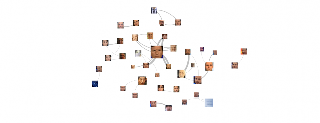
If you comment out the "connect to faces from previous frame" portion of the Perl script above, you'll get a graph that represents only faces that co-occur in the same frame. This will yield a visualization like the one below. Immediately clear is that a few of the detected faces are false positives, representing the limitations of the older face detection tool used. A number of the faces are actually the same person with slightly different head positioning, reflecting the limitations of pixel-level similarity grouping. It is clear that using a modern face extraction and grouping workflow that uses facial landmarks to group faces irrespective of pose would yield much more accurate results. But, even with these limitations, a number of key insights to the broadcast are visible, such as the figures cooccuring in the Tucker Carlson clips (these yield better grouping because they are filmed with the speakers looking directly into the camera from a short distance, yielding far less facial movement). Split-pane footage is less common on 60 Minutes, but these groupings capture several of the key exchanges.
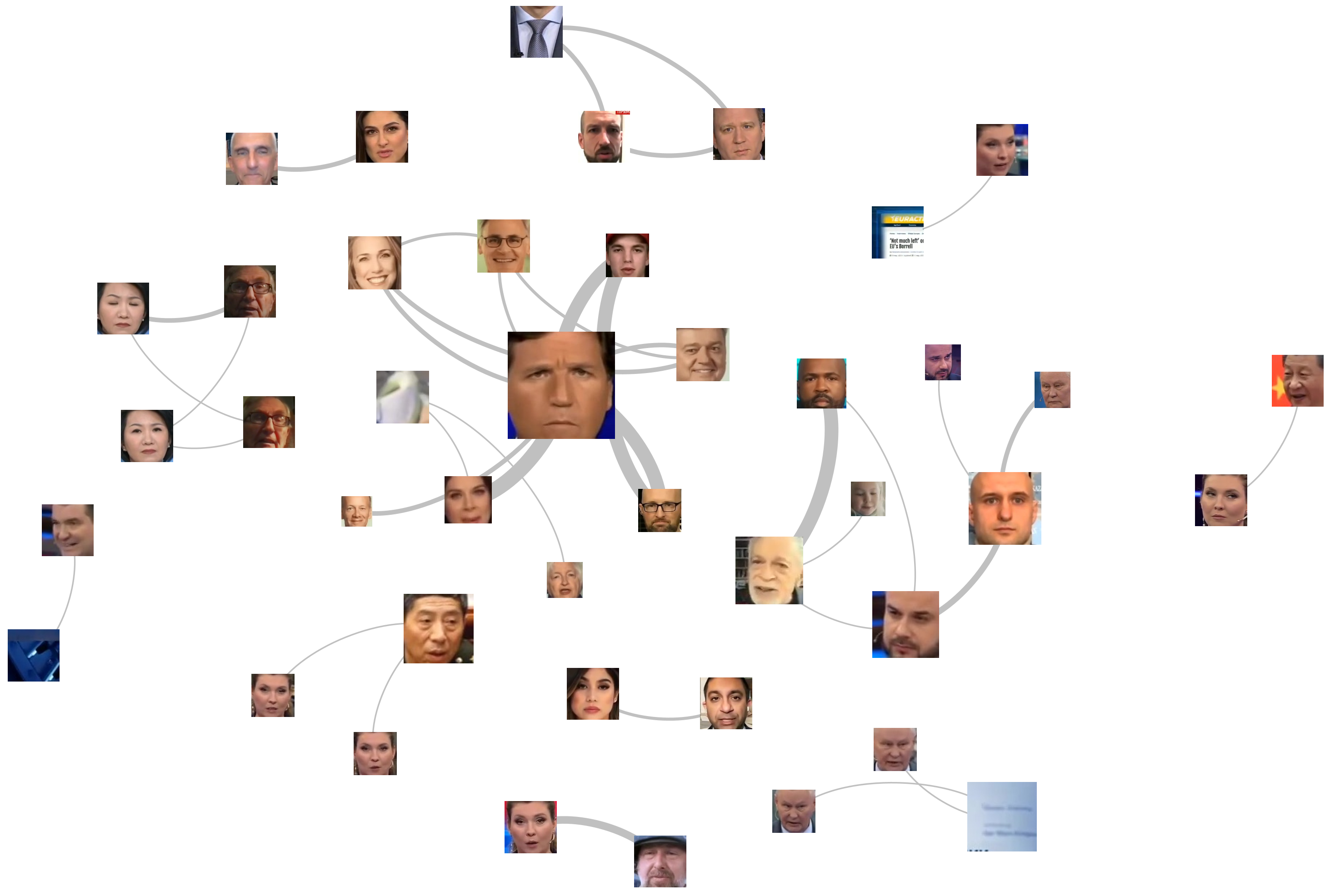
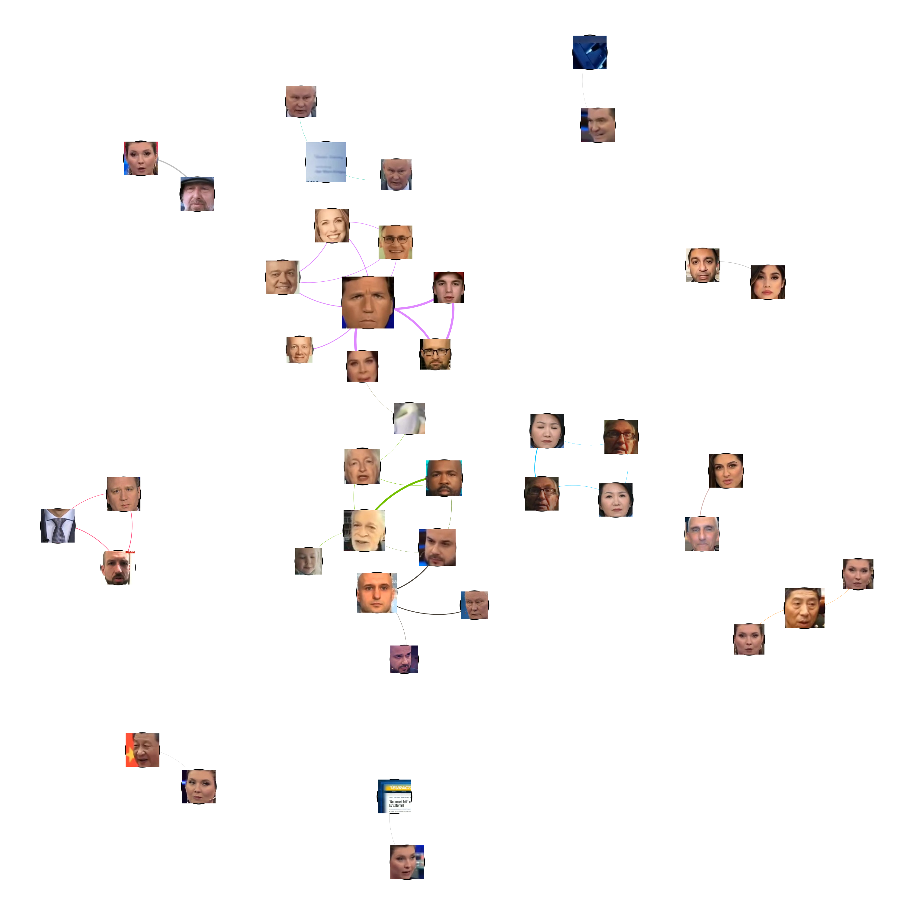
What if we leave the "connect to faces from previous frame" portion of the Perl script uncommented? This additionally groups faces that appeared within one frame of each other, capturing back-and-forth exchanges in addition to split-screen discussions. In addition to using PageRank to size the images, we also colorize them using Modularity to yield further clustering insights. The final graph can be seen below. Here several of the subclusters above can be seen to perform a single supercluster below, capturing the contextual framing of several of the exchanges.
The use of modern landmark-based facial extraction and clustering would vastly improve the accuracy of the results above, but even these basic results suggest tremendous potential. While the two visuals above are static images, more advanced visualizations could include clickable links to all of the clips where the faces cooccur, for example, allowing the graph to act as a jumping-off point for exploring the collection.
Note that there is no facial recognition performed in the workflow above. We are simply extracting faces and grouping them based on pixel-level similarity.
Despite its clear limitations, the pipeline above nonetheless offers a tantalizing glimpse at the incredible insights such analyses could offer in visualizing the narrative network of speakers across Russian television. Imagine the visualization above scaled up to the entire year-long archive of 60 Minutes monitored by the Internet Archive's TV News Archive or even scaled to all broadcasts across the five Russian channels it monitors. Expanding over time and across shows and even channels would allow a first glimpse at how Russian television leverages clips from Western television channels and its own stable of guests and speakers over time and across contexts and stories.
This analysis is part of an ongoing collaboration between the Internet Archive and its TV News Archive, the multi-party Media-Data Research Consortium and GDELT.