Earlier this week we visualized for the first time an entire day of global news coverage, including examining a sequence of three days in a row, while earlier today we showcased how our new visualization workflow can yield images that penetrate far more deeply into the innate structure of the global conversation. What would it look like to reexamine our sequence of three days of the global news landscape using this new visualization approach and even expand to a sample of six months?
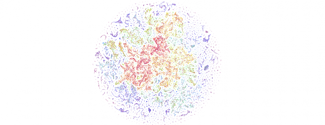
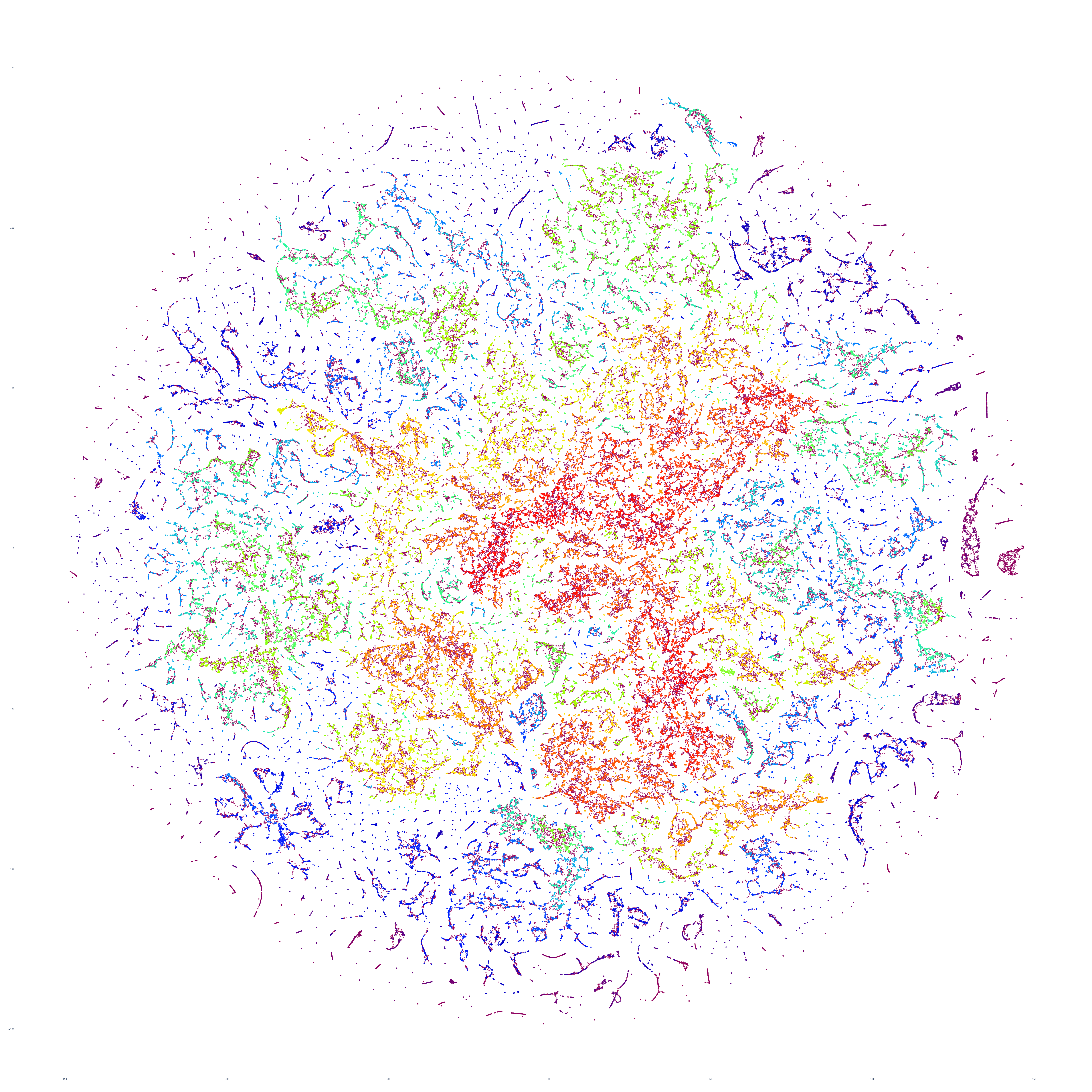
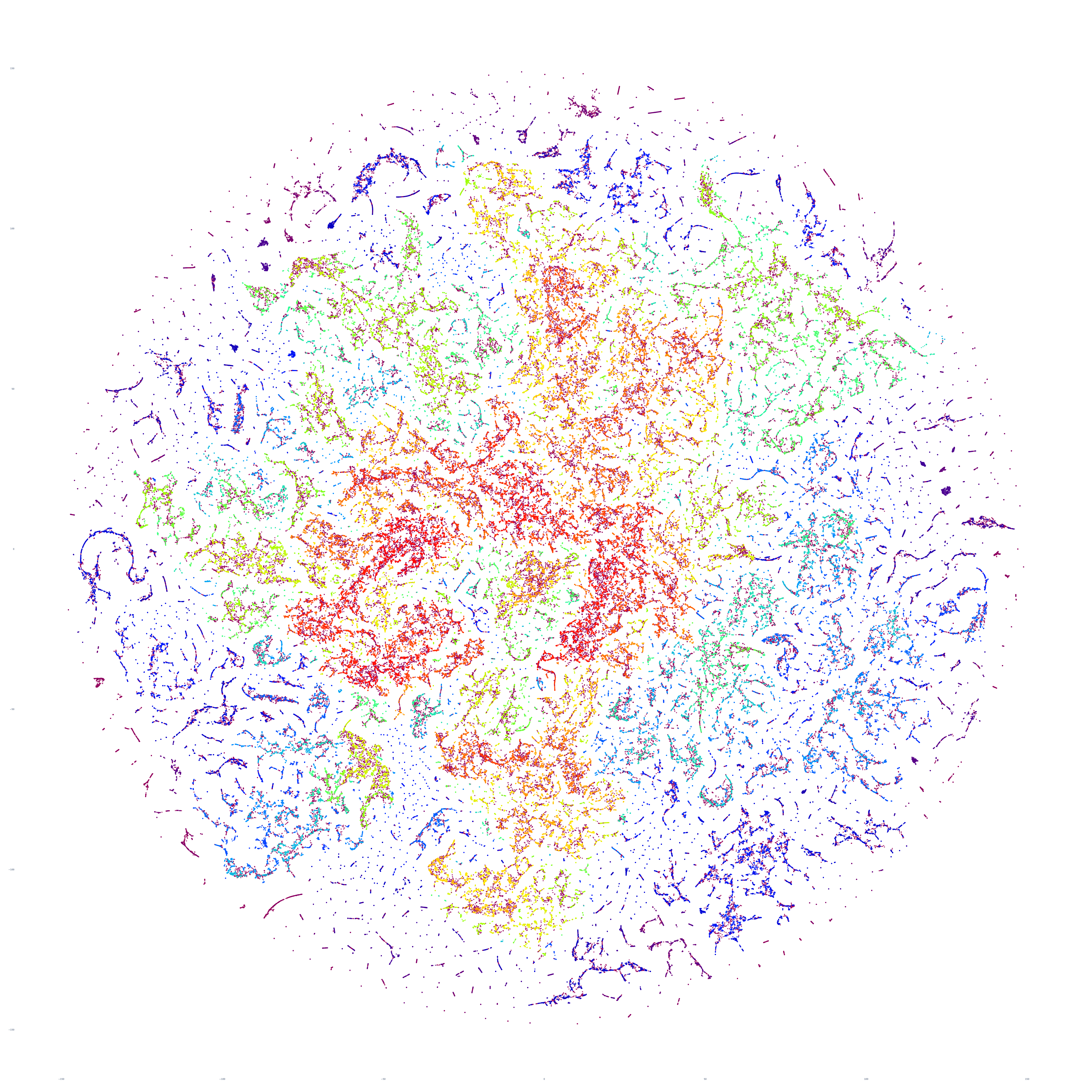
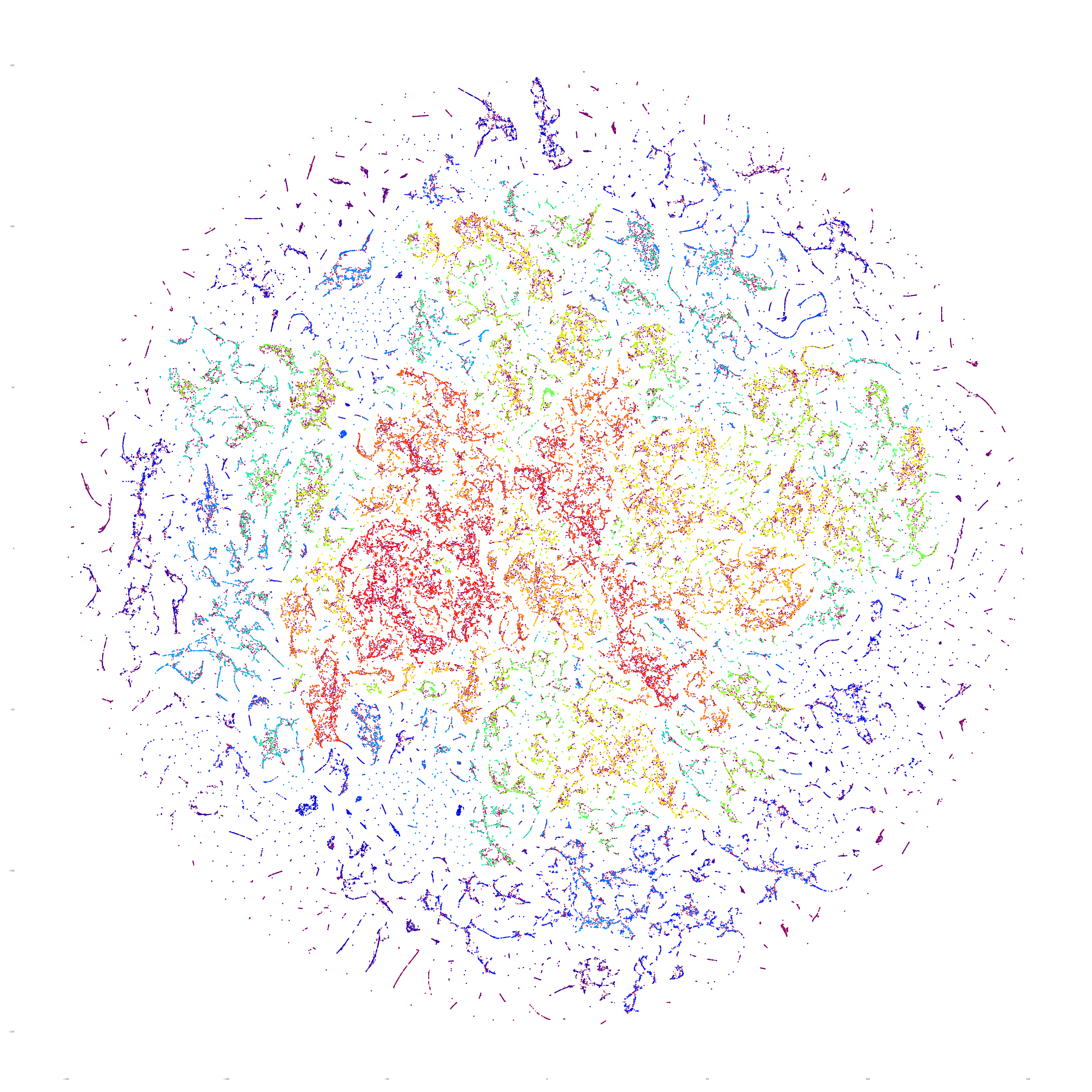
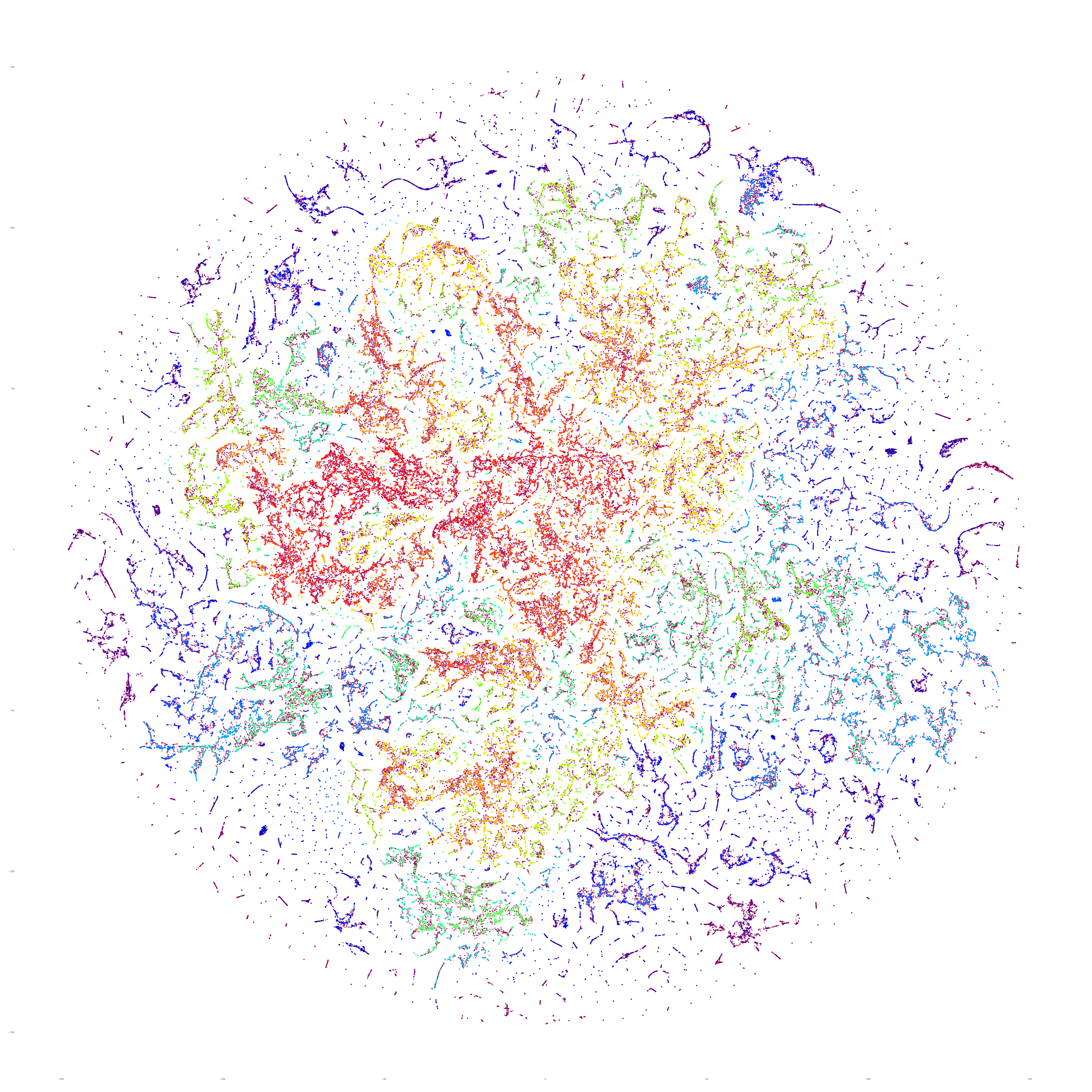
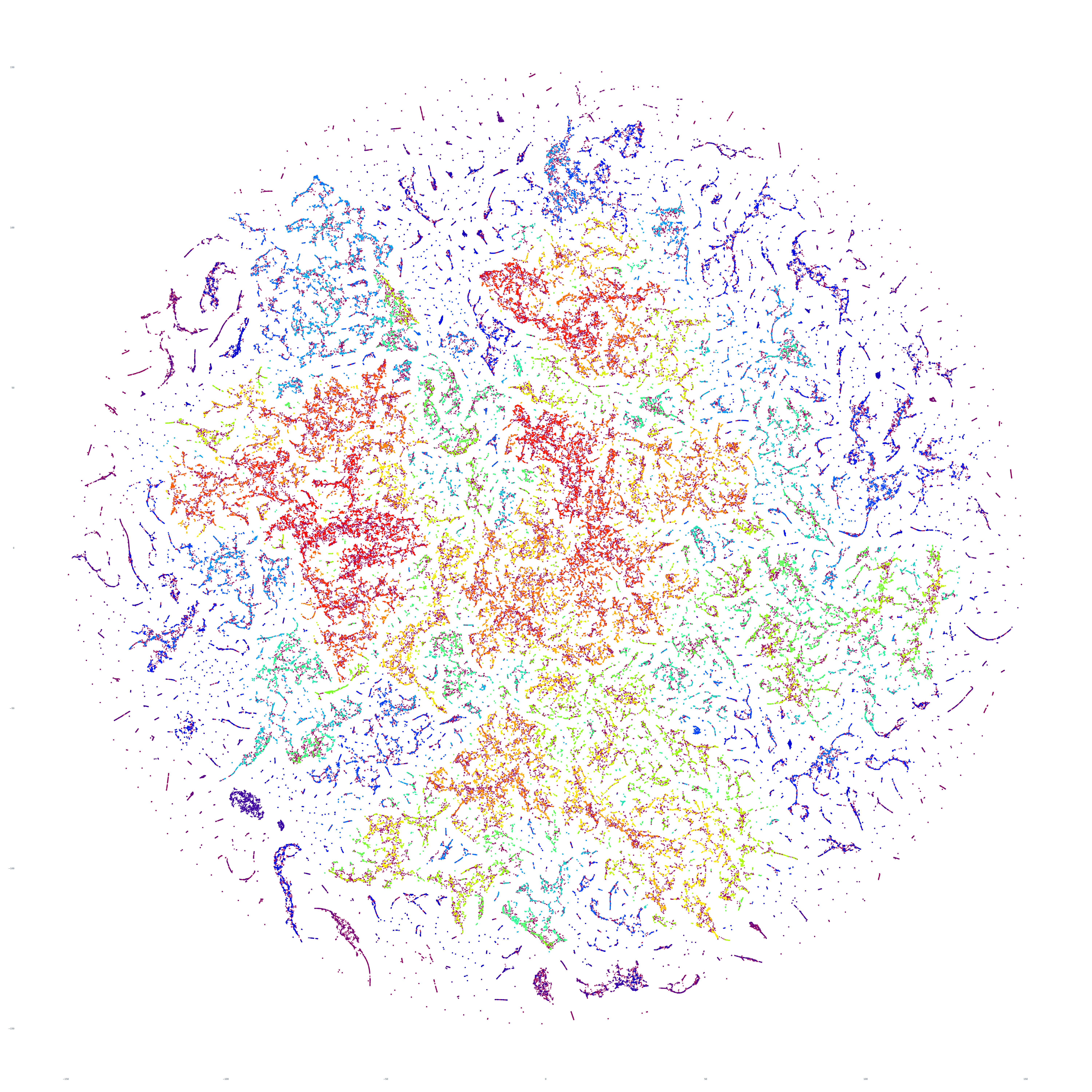
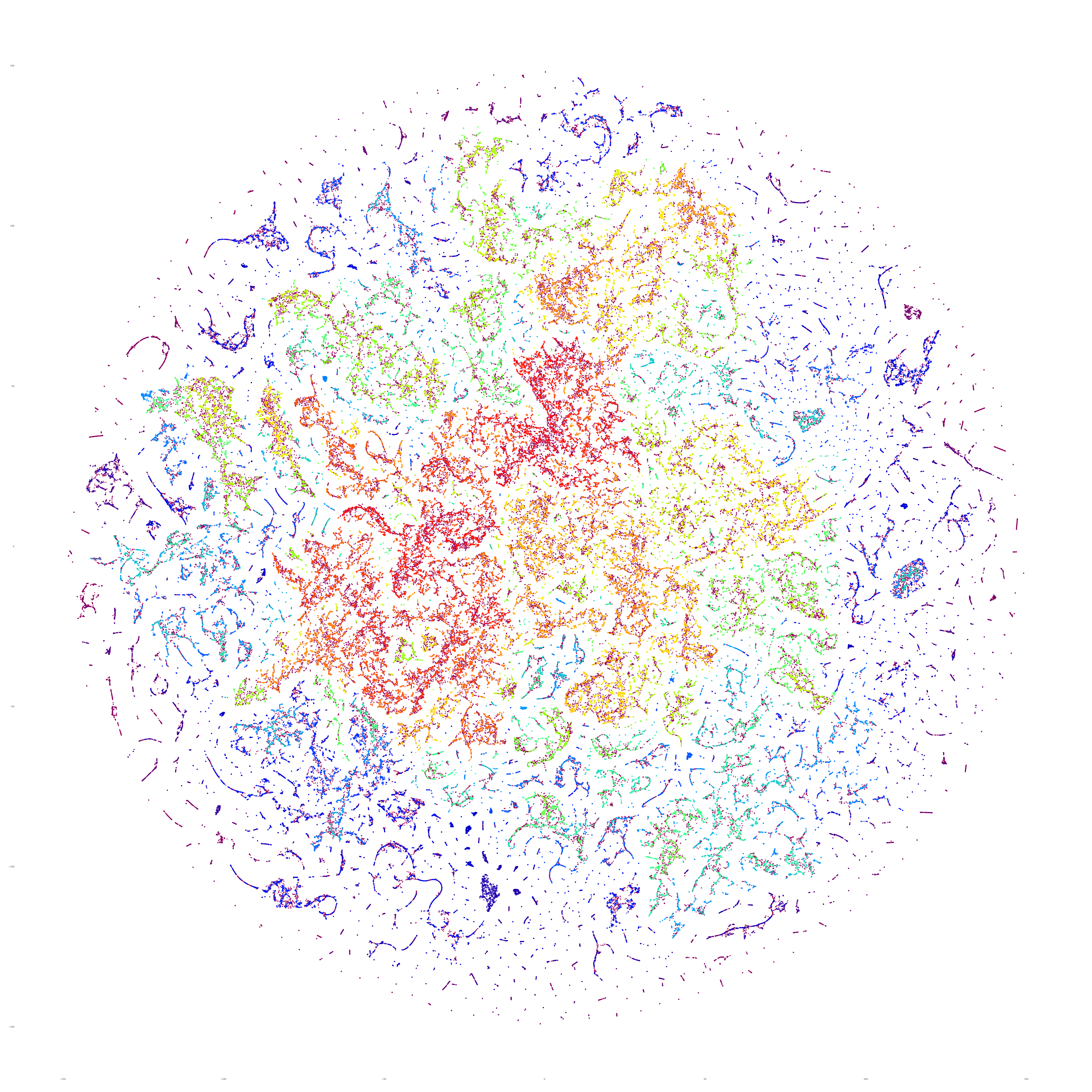
The end result is a sequence of images visualizing the global news landscape over four days (October 17-20, 2023) and one day each over six months (October 20, 2023, September 20, 2023, August 20, 2023, July 20, 2023, June 20, 2023, May 20, 2023). The images look strikingly similar: each of the sample days is, at first glance, nearly an exact duplicate of the others. Though, upon further examination, exhibits subtle differences, especially around the distribution and intersection of the diffuse superstructures. Do these images capture the true innate nature of our global media landscape, one defined by a near-constant structure that changes little day-by-day, or are the images below merely artifactual manifestations of the underlying algorithms used to produce them? Does the constant structure capture some kind of genuine momentum and affinity-based stable structure of the media landscape or does the combination of t-SNE, UMAP and HDBSCAN merely produce the exact same layout no matter the input? Could the choice of USEv4 embeddings, the use of machine translation into English or the use of document-level fulltext embeddings be artificially biasing the results? Clearly the dimensionality reduction of our preprocessing has an outsized influence on the resulting density and intricacy of the t-SNE layout, but which are more accurate reflections of the underlying patterns of the global media landscape: the diffuse point clouds of full-resolution t-SNE, or the tendril-like microstructures of low-dimensionality UMAP + t-SNE projection? All of these are questions we will be exploring in this series moving forward.
For the technically-minded, the full code is provided at the bottom of this page. We used UMAP to collapse the original 512-dimension USEv4 GSG fulltext document-level embeddings down to 10 dimensions, then used t-SNE to collapse to a 2D projection, which was provided to HDBSCAN for clustering and visualized directly as a scatterplot. Per our revised workflow from yesterday, we use the same t-SNE output for both HDBSCAN clustering and layout in order to allow HDBSCAN to capture and quantify to machine-friendly output the t-SNE projection so that clusters will be more visually aligned with layout, resulting in better alignment. To maintain computational tractability due to limitations in the underlying implementations and algorithms, we limited each image to a random sample of 350,000 articles from that day. In future we will be exploring GPU-accelerated and HPC implementations of the core algorithms and a variety of optimizations to our workflows to attempt to greatly accelerate both the scalability (to process the totality of a day's coverage rather than a random sample of it) and tractability (to process long sequences of months of the global conversation at a time).
October 20, 2023
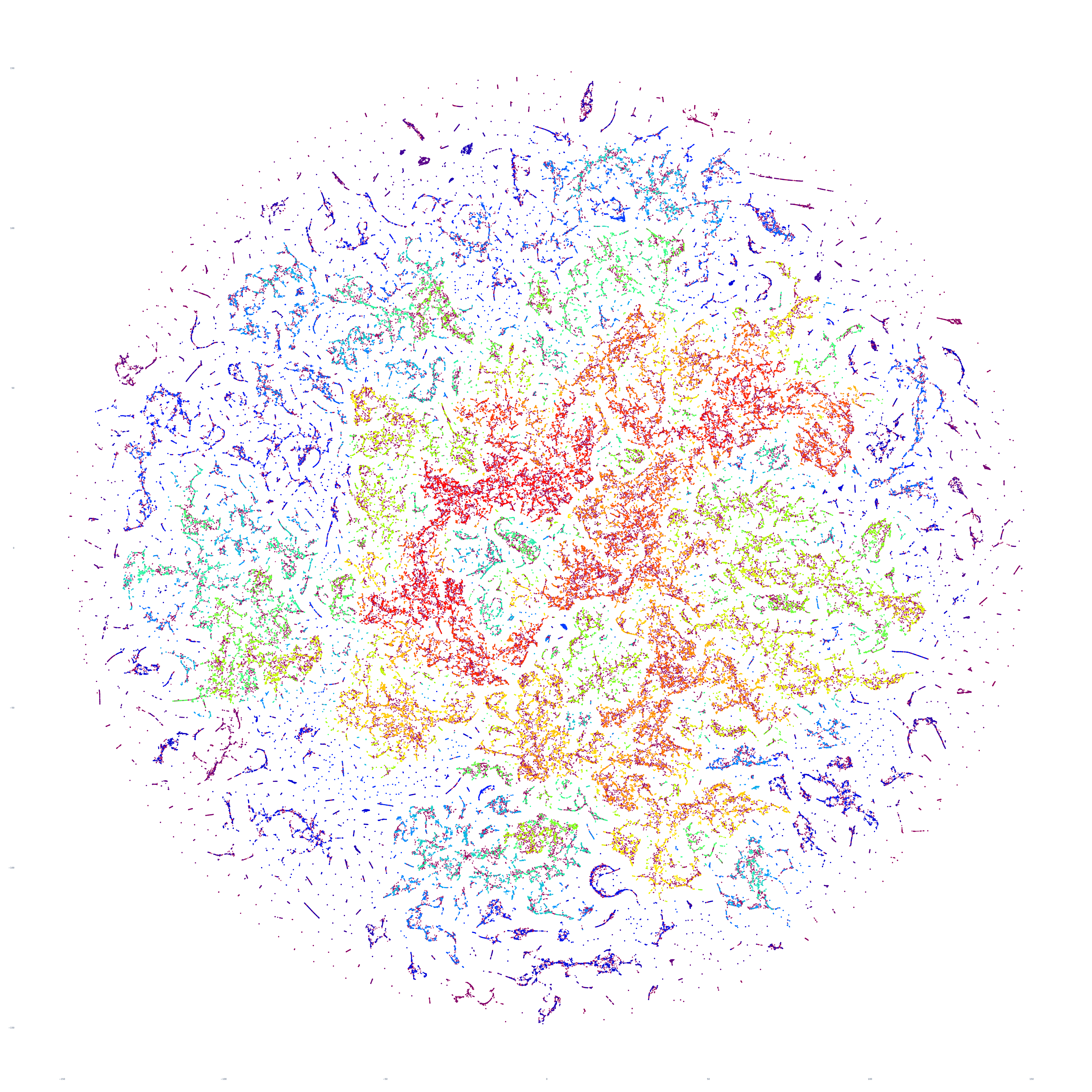
October 19, 2023
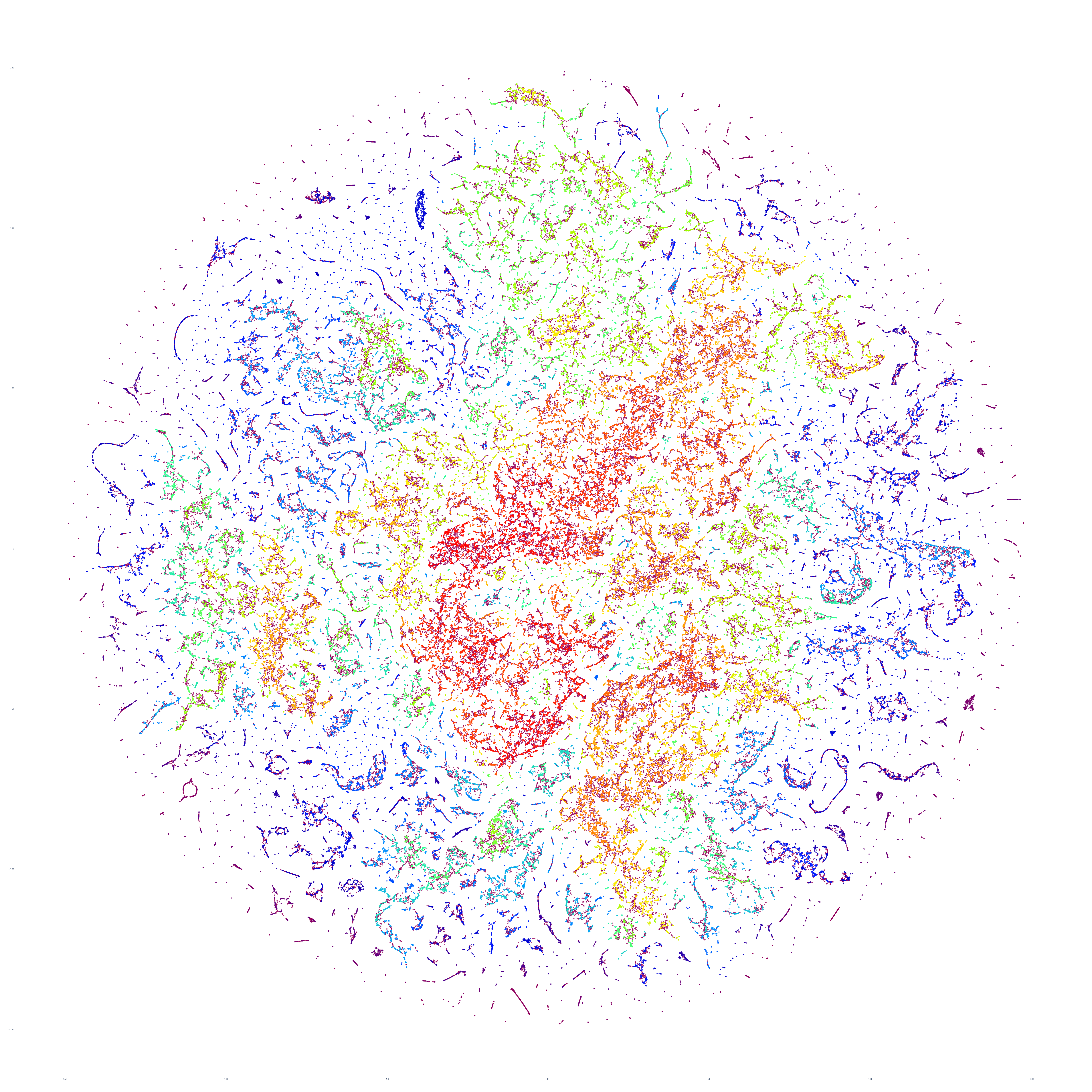
October 18, 2023
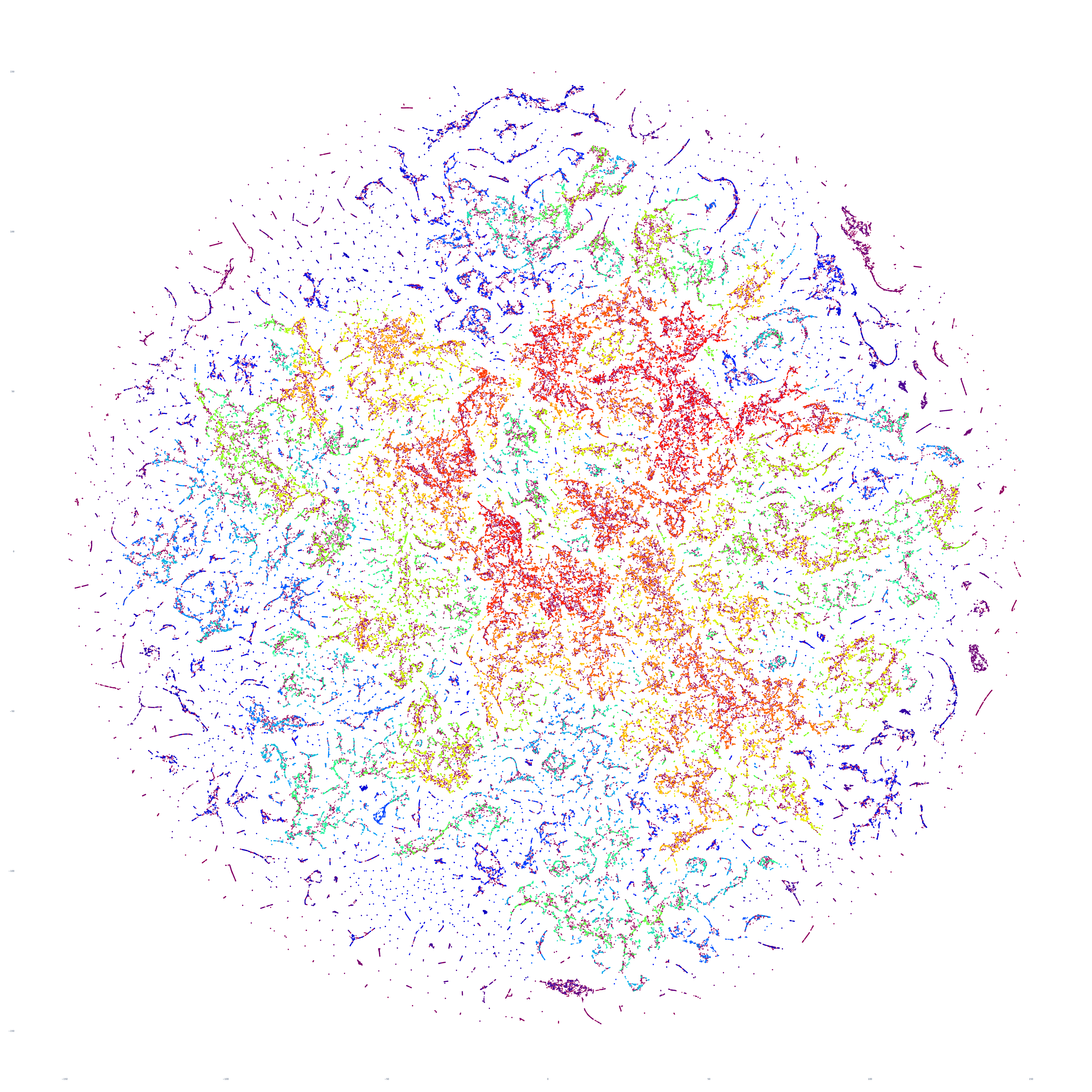
October 17, 2023
September 20, 2023
August 20, 2023
July 20, 2023
June 20, 2023
May 20, 2023
Technical Details
For those interested in replicating the results above, you can find the full code below.
Save the "collapse.pl" script from our original experiment, then run a sequence of commands like the following:
rm -rf ./CACHE/; mkdir CACHE
#DOWNLOAD: https://storage.googleapis.com/data.gdeltproject.org/gdeltv3/gsg_docembed/20230920*.gsg.docembed.json.gz ./CACHE/
time find ./CACHE/*.gz | parallel --eta 'pigz -d {}'
time ./collapse.pl
time shuf -n 350000 MASTER.json > MASTER.sample.json.350k
time python3 ./run.py ./2023-10-sept20gsg-350k-umaptosne10hdbscan-tsnareduced10paired ./MASTER.sample.json.350k

rm -rf ./CACHE/; mkdir CACHE
#DOWNLOAD: https://storage.googleapis.com/data.gdeltproject.org/gdeltv3/gsg_docembed/20230820*.gsg.docembed.json.gz ./CACHE/
time find ./CACHE/*.gz | parallel --eta 'pigz -d {}'
time ./collapse.pl
time shuf -n 350000 MASTER.json > MASTER.sample.json.350k
time python3 ./run.py ./2023-10-aug20gsg-350k-umaptosne10hdbscan-tsnareduced10paired ./MASTER.sample.json.350k

rm -rf ./CACHE/; mkdir CACHE
#DOWNLOAD: https://storage.googleapis.com/data.gdeltproject.org/gdeltv3/gsg_docembed/20230720*.gsg.docembed.json.gz ./CACHE/
time find ./CACHE/*.gz | parallel --eta 'pigz -d {}'
time ./collapse.pl
time shuf -n 350000 MASTER.json > MASTER.sample.json.350k
time python3 ./run.py ./2023-10-july20gsg-350k-umaptosne10hdbscan-tsnareduced10paired ./MASTER.sample.json.350k
We ran these on a 64-core GCE N1 VM with 400GB RAM. Each run took around 35 minutes or so. You can see a sample run below:
time python3 ./runk.py ./2023-10-oct20gsg-350k-umaptosne10hdbscan-tsnareduced10paired ./MASTER.sample.json.350k
UMAP(min_dist=0.0, n_components=10, n_neighbors=30, verbose=True)
Fri Nov  3 20:35:49 2023 Construct fuzzy simplicial set
Fri Nov  3 20:35:50 2023 Finding Nearest Neighbors
Fri Nov  3 20:35:50 2023 Building RP forest with 35 trees
Fri Nov  3 20:36:00 2023 NN descent for 18 iterations
         1  /  18
         2  /  18
         3  /  18
         4  /  18
         5  /  18
        Stopping threshold met -- exiting after 5 iterations
Fri Nov  3 20:37:29 2023 Finished Nearest Neighbor Search
Fri Nov  3 20:37:37 2023 Construct embedding
Epochs completed:   0%|                                                                                                    0/200 [00:00completed  0  /  200 epochs
Epochs completed:  10%| █████████▋                                                                                        20/200 [00:21completed  20  /  200 epochs
Epochs completed:  20%| ███████████████████▍                                                                              40/200 [00:44completed  40  /  200 epochs
Epochs completed:  30%| █████████████████████████████                                                                     60/200 [01:08completed  60  /  200 epochs
Epochs completed:  40%| ██████████████████████████████████████▊                                                           80/200 [01:31completed  80  /  200 epochs
Epochs completed:  50%| ████████████████████████████████████████████████                                                 100/200 [01:55completed  100  /  200 epochs
Epochs completed:  60%| █████████████████████████████████████████████████████████▌                                       120/200 [02:19completed  120  /  200 epochs
Epochs completed:  70%| ███████████████████████████████████████████████████████████████████▏                             140/200 [02:42completed  140  /  200 epochs
Epochs completed:  80%| ████████████████████████████████████████████████████████████████████████████▊                    160/200 [03:06completed  160  /  200 epochs
Epochs completed:  90%| ██████████████████████████████████████████████████████████████████████████████████████▍          180/200 [03:29completed  180  /  200 epochs
Epochs completed: 100%| ████████████████████████████████████████████████████████████████████████████████████████████████ 200/200 [03:53]
Fri Nov  3 20:53:11 2023 Finished embedding
Dimensionality Reduction: : 60241.761098507 seconds
HDBSCAN: : 25.449612440999772 seconds
Clusters: [   -1     0     1 ... 16249 16250 16251]
Num Clusters: 16253
Noise Articles: 60959
Wrote Clusters
Layout (TSNE): 5.3085001127328724e-05 seconds
Render: 0.9744974019995425 seconds

real    34m52.026s
The final script used is the following, modified from our original script and our subsequent optimizations.
#########################
#LOAD THE EMBEDDINGS...

import numpy as np
import matplotlib.pyplot as plt
from PIL import Image
import jsonlines
import multiprocessing
import sys

# Load the JSON file containing embedding vectors
def load_json_embeddings(filename):
    embeddings = []
    titles = []
    langs = []
    with jsonlines.open(filename) as reader:
        for line in reader:
            embeddings.append(line["embed"])
            titles.append(line["title"])
            langs.append(line["lang"])
    return np.array(embeddings), titles, langs

#json_file = 'MASTER.sample.json.500'
json_file = sys.argv[2]
embeddings, titles, langs = load_json_embeddings(json_file)
len(embeddings)

import hdbscan
import umap
from sklearn.decomposition import PCA
from sklearn.manifold import TSNE
import time
clusters = []
embeddings_reduced = []
def cluster_embeddings(embeddings, min_cluster_size=5):
    global clusters, embeddings_reduced
    start_time = time.process_time()
    #embeddings_reduced = PCA(n_components=10, random_state=42).fit_transform(embeddings)
    embeddings_reduced = umap.UMAP(n_neighbors=30,min_dist=0.0,n_components=10,verbose=True).fit_transform(embeddings)
    tsne = TSNE(n_components=2, random_state=42)
    embeddings_reduced = tsne.fit_transform(embeddings_reduced)
    end_time = time.process_time()
    elapsed_time = end_time - start_time
    print(f"Dimensionality Reduction: : {elapsed_time} seconds")
    start_time = time.process_time()
    clusterer = hdbscan.HDBSCAN(min_cluster_size=min_cluster_size, core_dist_n_jobs = multiprocessing.cpu_count())
    clusters = clusterer.fit_predict(embeddings_reduced)
    end_time = time.process_time()
    elapsed_time = end_time - start_time
    print(f"HDBSCAN: : {elapsed_time} seconds")
    #return clusters

#cluster...
cluster_embeddings(embeddings, 5)

#output some basic statistics...
unique_clusters = np.unique(clusters)
print("Clusters: " + str(unique_clusters))
print("Num Clusters: " + str(len(unique_clusters)))
cnt_noise = np.count_nonzero(clusters == -1)
print("Noise Articles: " + str(cnt_noise))

#write the output...
with open(sys.argv[1] + '.tsv', 'w', encoding='utf-8') as tsv_file:
    for cluster_id, title, lang in zip(clusters, titles, langs):
        tsv_file.write(f"{cluster_id}\t{title}\t{lang}\n")
print("Wrote Clusters")

#########################
#VISUALIZE...

from sklearn.manifold import TSNE
from sklearn.decomposition import PCA
import plotly.graph_objs as graph
import plotly.io as pio

def plotPointCloud(embeddings, clusters, titles, langs, title, algorithm):
    if (algorithm == 'PCA'):
        start_time = time.process_time()
        pca = PCA(n_components=2, random_state=42)
        embeds = pca.fit_transform(embeddings)
        end_time = time.process_time()
        elapsed_time = end_time - start_time
        print(f"Layout (PCA): {elapsed_time} seconds")
    if (algorithm == 'TSNE'):
        start_time = time.process_time()
        tsne = TSNE(n_components=2, random_state=42)
        #embeds = tsne.fit_transform(embeddings)
        embeds = embeddings_reduced
        end_time = time.process_time()
        elapsed_time = end_time - start_time
        print(f"Layout (TSNE): {elapsed_time} seconds")

    start_time = time.process_time()
    trace = graph.Scatter(
        x=embeds[:, 0],
        y=embeds[:, 1],
        marker=dict(
            size=6,
            #color=np.arange(len(embeds)), #color randomly
            color=clusters, #color via HDBSCAN clusters
            colorscale='Rainbow',
            opacity=0.8
        ),
        #text = langs,
        #text = titles,
        #text = [title[:20] for title in titles],
        hoverinfo='text',
        #mode='markers+text',
        mode='markers',
        textposition='bottom right'
    )

    layout = graph.Layout(
        #title=title,
        xaxis=dict(title=''),
        yaxis=dict(title=''),
        height=6000,
        width=6000,
        plot_bgcolor='rgba(255,255,255,255)',
        hovermode='closest',
        hoverlabel=dict(bgcolor="black", font_size=14)
    )

    fig = graph.Figure(data=[trace], layout=layout)
    fig.update_layout(autosize=True)

    # Save the figure as a PNG image
    pio.write_image(fig, sys.argv[1] + '.png', format='png')
    end_time = time.process_time()
    elapsed_time = end_time - start_time
    print(f"Render: {elapsed_time} seconds")

# Call the function with your data
#clusters = []
plotPointCloud(embeddings, clusters, titles, langs, 'Title', 'TSNE')
#########################