This week's visualizations of an entire day of global news coverage were limited by one key factor: computational tractability. Even running on a 64-core GCE N1 VM with 400GB of RAM, each rendering took a considerable amount of time and the final renderings were limited to an upper bound of a 350K random sample rather than the full dataset due to limitations in the underlying algorithm implementations. How might one major set of optimizations help accelerate these visualizations and what tradeoffs might they present?
Our visualizations yesterday made use of UMAP dimensionality reduction to reduce the 512-dimension USEv4 embedding vectors down to 10 dimensions to make HDBSCAN clustering computationally feasible. How does UMAP compare with PCA in terms of the impact they have on the resulting cluster formation and visualizations? In yesterday's visualizations, we used UMAP only for HDBSCAN and then reverted to using the full-resolution 512-dimension vectors for our t-SNE layout. To what degree would using the reduced embeddings accelerate the t-SNE layout and where are we spending the majority of our time?
The end result is that contrary to widely-touted recommendation in some quarters that PCA executes many times faster than UMAP, in our real-world experiments below we find that the gains, at least for USEv4's 512-dimension vectors, are far more modest, yielding just a few minutes in most cases, though with greater impact for larger datasets. Worse, the PCA-reduced results are nearly meaningless, causing HDBSCAN to cluster nearly the entire graph into the noise category due to PCA's global-structure focus. In contrast, UMAP yields strong results as we found in our original experiment. In terms of accelerating the t-SNE layout process, using the UMAP-reduced embeddings, rather than the original full-resolution embeddings yields modest speed improvements, but has a fascinating side effect: it causes t-SNE to replace the diffuse point clouds seen in our original graphs with intricate tightly-woven tendrils of interconnected clusters, even for articles marked as "noise" by HDBSCAN. The resulting visualizations from full-resolution and reduced-resolution t-SNE layouts take roughly similar execution times, but the reduced t-SNE layouts produce vastly more understandable structure that tightly organizes the global media landscape. Whether this additional structure is meaningful and whether it yields better or worse understanding than the diffuse point clouds (especially whether the actual underlying semantic structure in those areas is legitimately more diffuse or structured) is an area for additional research. Comparing different levels of dimensionality reduction, the macro-level visualizations change little across different dimensionality levels, with the exception of UMAP-based 2D projection, suggesting that execution time considerations and available CPU resources (due to the different levels of multicore parallelism available in each stage) may be able to play a larger role in selecting the ideal settings – though key questions remain about how these choices impact downstream cluster utility.
You can see the timing breakdowns below. Note that we use wallclock time for the overall time and Python's "time.process_time()" for the task-level timings, which summarizes the total time across all cores, which is why on this 64-core VM those times are substantially higher than the wallclock time.
Here are the results for using PCA dimensionality reduction to 10 dimensions and t-SNE layout using the full-resolution 512-dimension vectors. We can immediately see that the largest amount of time is spent in the t-SNE layout stage and that it leverages all 64-cores to achieve even these lengthy runtimes:
time python3 ./runn.py ./output-500-pcahdbscan-tsnafull ./MASTER.sample.json.500
PCA: : 2.428847918999999 seconds
HDBSCAN: : 3.195304661999998 seconds
Num Clusters: 3
Noise Articles: 220
Layout (TSNE): 5021.147535501999 seconds
Render: 1.1501990320002733 seconds
#1m27.544s

time python3 ./runn.py ./output-10k-pcahdbscan-tsnafull ./MASTER.sample.json.10k
PCA: 11.469120534999998 seconds
HDBSCAN: : 6.248807965999994 seconds
Num Clusters: 86
Noise Articles: 8266
Layout (TSNE): 10239.753743214 seconds
Render: 0.9250311149990011 seconds
#2m56.447s

time python3 ./runn.py ./output-100k-pcahdbscan-tsnafull ./MASTER.sample.json.100k
PCA: : 88.013860348 seconds
HDBSCAN: : 53.17140504599999 seconds
Num Clusters: 1539
Noise Articles: 82202
Layout (TSNE): 13126.031354806999 seconds
Render: 1.1888463730010699 seconds
#8m3.757s

time python3 ./runn.py ./output-200k-pcahdbscan-tsnafull ./MASTER.sample.json.200k
PCA: : 138.27123590800002 seconds
HDBSCAN: : 204.663445835 seconds
Num Clusters: 3561
Noise Articles: 155658
Layout (TSNE): 18653.367705542 seconds
Render: 0.8991585709991341 seconds
#16m54.485s

time python3 ./runn.py ./output-350k-pcahdbscan-tsnafull ./MASTER.sample.json.350k
PCA: : 185.823394168 seconds
HDBSCAN: : 437.51286312400003 seconds
Num Clusters: 6668
Noise Articles: 261038
Layout (TSNE): 31658.361666378998 seconds
Render: 0.9239981770006125 seconds
#27m35.886s
Here are the results for using PCA dimensionality reduction to 10 dimensions and t-SNE layout using the same reduced 10-dimension vectors. We can see that reducing the dimensionality of the vectors for t-SNE only speeds things up by a few minutes other than for the largest dataset where it has a more measurable impact:
time python3 ./runn.py ./output-500-pcahdbscan-tsnareduced10 ./MASTER.sample.json.500
PCA: : 2.3914137330000003 seconds
HDBSCAN: : 2.2154759669999997 seconds
Num Clusters: 3
Noise Articles: 220
Wrote Clusters
Layout (TSNE): 3143.357393109 seconds
Render: 1.2123616369999581 seconds
#0m57.908s

time python3 ./runn.py ./output-10k-pcahdbscan-tsnareduced10 ./MASTER.sample.json.10k
PCA: : 12.670889239000001 seconds
HDBSCAN: : 6.556422175000002 seconds
Num Clusters: 86
Noise Articles: 8266
Wrote Clusters
Layout (TSNE): 9172.155809331001 seconds
Render: 1.1619373419998738 seconds
#2m44.259s
time python3 ./runn.py ./output-100k-pcahdbscan-tsnareduced10 ./MASTER.sample.json.100k
PCA: : 82.800410946 seconds
HDBSCAN: : 53.497904571999996 seconds
Num Clusters: 1539
Noise Articles: 82202
Wrote Clusters
Layout (TSNE): 12909.733578517 seconds
Render: 1.1690794980004284 seconds
#9m8.552s

time python3 ./runn.py ./output-200k-pcahdbscan-tsnareduced10 ./MASTER.sample.json.200k
PCA: : 137.806066569 seconds
HDBSCAN: : 204.25508139299998 seconds
Num Clusters: 3561
Noise Articles: 155658
Wrote Clusters
Layout (TSNE): 15502.679567828001 seconds
Render: 1.2023969459987711 seconds
#20m29.470s

time python3 ./runn.py ./output-350k-pcahdbscan-tsnareduced10 ./MASTER.sample.json.350k
PCA: : 188.180185 seconds
HDBSCAN: : 430.095274092 seconds
Num Clusters: 6668
Noise Articles: 261038
Wrote Clusters
Layout (TSNE): 21291.865324438997 seconds
Render: 0.9988922129996354 seconds
#41m17.613s
What about repeating our exact workflow from yesterday? This uses UMAP dimensionality reduction to 10 dimensions and t-SNE layout using the raw 512-dimension vectors. This is only slightly slower than using PCA, suggesting that, contrary to some touted recommendations that PCA is several times faster than UMAP, the speed improvements are far more modest:
time python3 ./runn.py ./output-500-umaphdbscan-tsnafull ./MASTER.sample.json.500
UMAP: : 368.454166479 seconds
HDBSCAN: : 0.8235538530000213 seconds
Num Clusters: 16
Noise Articles: 172
Layout (TSNE): 4124.352307461 seconds
Render: 1.1703988250001203 seconds
#1m28.217s

time python3 ./runn.py ./output-10k-umaphdbscan-tsnafull ./MASTER.sample.json.10k
UMAP: : 1232.297609941 seconds
HDBSCAN: : 0.4298013449999871 seconds
Num Clusters: 289
Noise Articles: 4406
Layout (TSNE): 10092.327194671 seconds
Render: 1.2001219960002345 seconds
#3m40.956s

time python3 ./runn.py ./output-100k-umaphdbscan-tsnafull ./MASTER.sample.json.100k
UMAP: : 5882.439154004 seconds
HDBSCAN: : 13.227559089999886 seconds
Num Clusters: 2860
Noise Articles: 44973
Layout (TSNE): 13197.688294931002 seconds
Render: 0.9783284889999777 seconds
#9m59.227s

time python3 ./runn.py ./output-200k-umaphdbscan-tsnafull ./MASTER.sample.json.200k
UMAP: : 18389.744759906 seconds
HDBSCAN: : 35.15340755699799 seconds
Num Clusters: 5765
Noise Articles: 84240
Layout (TSNE): 18575.747295277004 seconds
Render: 1.0938486810046015 seconds
#20m8.909s

time python3 ./runn.py ./output-350k-umaphdbscan-tsnafull ./MASTER.sample.json.350k
UMAP: : 43686.995292346 seconds
HDBSCAN: : 77.35459611599799 seconds
Num Clusters: 10268
Noise Articles: 142510
Layout (TSNE): 31135.895989659002 seconds
Render: 1.388311809001607 seconds
#40m37.998s
What about repeating our exact workflow from yesterday? This uses UMAP dimensionality reduction to 10 dimensions and t-SNE layout using the same reduced 10-dimension vectors. As before, we see that the speedup is fairly modest:
time python3 ./runn.py ./output-500-umaphdbscan-tsnareduced10 ./MASTER.sample.json.500
UMAP: : 598.419491917 seconds
HDBSCAN: : 0.7507073090000631 seconds
Num Clusters: 16
Noise Articles: 183
Wrote Clusters
Layout (TSNE): 1266.0424988309999 seconds
Render: 1.3197430190000432 seconds
#0m46.687s

time python3 ./runn.py ./output-10k-umaphdbscan-tsnareduced10 ./MASTER.sample.json.10k
UMAP: : 1209.028011256 seconds
HDBSCAN: : 0.4505578350001542 seconds
Num Clusters: 276
Noise Articles: 4072
Layout (TSNE): 10004.430830412 seconds
Render: 1.187103238000418 seconds
#3m39.816s

time python3 ./runn.py ./output-100k-umaphdbscan-tsnareduced10 ./MASTER.sample.json.100k
UMAP: : 5870.5331127419995 seconds
HDBSCAN: : 13.17594723900038 seconds
Num Clusters: 2872
Noise Articles: 44164
Layout (TSNE): 12285.250289804 seconds
Render: 1.1833040329984215 seconds
#9m25.074s

time python3 ./runn.py ./output-200k-umaphdbscan-tsnareduced10 ./MASTER.sample.json.200k
UMAP: : 16131.221890108 seconds
HDBSCAN: : 37.84411430199907 seconds
Num Clusters: 5755
Noise Articles: 84963
Layout (TSNE): 14462.390557632001 seconds
Render: 1.2095746349987166 seconds
#18m45.838s

time python3 ./runn.py ./output-350k-umaphdbscan-tsnareduced10 ./MASTER.sample.json.350k
UMAP: : 37198.735697563 seconds
HDBSCAN: : 72.86624144199595 seconds
Num Clusters: 10341
Noise Articles: 144567
Layout (TSNE): 19286.276156513 seconds
Render: 1.0964710260013817 seconds
#36m37.211s
Finally, what if we halve the final reduced dimensions from 10 to 5? We'll use UMAP to reduce the embeddings to 5 dimensions instead of 10 for HDBSCAN, while t-SNE layout will still use the original full-resolution embeddings. This does accelerate the HDBSCAN processing, but the speedup is less noticeable given that the majority of the runtime is spent in the t-SNE layout:
time python3 ./runn.py ./output-500-umap5hdbscan-tsnafull ./MASTER.sample.json.500
UMAP: : 470.496131752 seconds
HDBSCAN: : 0.013146705999986352 seconds
Num Clusters: 17
Noise Articles: 185
Layout (TSNE): 2542.394735153 seconds
Render: 1.2131023789997926 seconds
#1m4.738s

time python3 ./runn.py ./output-10k-umap5hdbscan-tsnafull ./MASTER.sample.json.10k
UMAP: : 1523.339983019 seconds
HDBSCAN: : 0.3251564800000324 seconds
Num Clusters: 280
Noise Articles: 3777
Layout (TSNE): 10200.13727831 seconds
Render: 1.1970147199990606 seconds
#3m48.241s

time python3 ./runn.py ./output-100k-umap5hdbscan-tsnafull ./MASTER.sample.json.100k
UMAP: : 6030.816045222 seconds
HDBSCAN: : 8.934514333000152 seconds
Num Clusters: 2791
Noise Articles: 43781
Layout (TSNE): 13110.000106106001 seconds
Render: 1.209525507001672 seconds
#9m55.496s

time python3 ./runn.py ./output-200k-umap5hdbscan-tsnafull ./MASTER.sample.json.200k
UMAP: : 18515.067846399 seconds
HDBSCAN: : 18.549581690000196 seconds
Num Clusters: 5645
Noise Articles: 83175
Layout (TSNE): 18684.747698655996 seconds
Render: 1.2559453029971337 seconds
#20m1.666s

time python3 ./runn.py ./output-350k-umap5hdbscan-tsnafull ./MASTER.sample.json.350k
UMAP: : 54159.975082827994 seconds
HDBSCAN: : 36.07115693599917 seconds
Num Clusters: 10179
Noise Articles: 140631
Layout (TSNE): 31377.275541920004 seconds
Render: 1.1267633289971855 seconds
#43m17.834s
Let's repeat the process by using the UMAP-reduced 5-dimension embeddings for both HDBSCAN and the t-SNE layout. This yields a measurable speedup across the board.
time python3 ./runn.py ./output-500-umap5hdbscan-tsnareduced5 ./MASTER.sample.json.500
UMAP: : 70.59044030000001 seconds
HDBSCAN: : 0.9316715310000063 seconds
Num Clusters: 16
Noise Articles: 171
Wrote Clusters
Layout (TSNE): 80.408629557 seconds
Render: 1.1585667530000023 seconds
#0m18.249s

time python3 ./runn.py ./output-10k-umap5hdbscan-tsnareduced5 ./MASTER.sample.json.10k
UMAP: : 872.813494192 seconds
HDBSCAN: : 0.31622454399996514 seconds
Num Clusters: 305
Noise Articles: 4202
Wrote Clusters
Layout (TSNE): 1104.881352882 seconds
Render: 1.1129478450000079 seconds
#1m12.285s

time python3 ./runn.py ./output-100k-umap5hdbscan-tsnareduced5 ./MASTER.sample.json.100k
UMAP: : 4547.908635771 seconds
HDBSCAN: : 8.437193822000154 seconds
Num Clusters: 2815
Noise Articles: 43241
Wrote Clusters
Layout (TSNE): 3174.993998594 seconds
Render: 1.0414020039997922 seconds
#6m16.179s

time python3 ./runn.py ./output-200k-umap5hdbscan-tsnareduced5 ./MASTER.sample.json.200k
UMAP: : 17211.637760808 seconds
HDBSCAN: : 16.488291566001863 seconds
Num Clusters: 5748
Noise Articles: 84971
Wrote Clusters
Layout (TSNE): 5928.9593736940005 seconds
Render: 1.1873650999987149 seconds
#15m1.042s

time python3 ./runn.py ./output-350k-umap5hdbscan-tsnareduced5 ./MASTER.sample.json.350k
UMAP: : 48287.342618541996 seconds
HDBSCAN: : 33.55415799700131 seconds
Num Clusters: 10185
Noise Articles: 142834
Wrote Clusters
Layout (TSNE): 10488.731985585 seconds
Render: 1.1234332350068144 seconds
#33m57.061s
What if we increase the number of dimensions up to 25? We'll use UMAP to reduce the 512-dimension USEv4 embeddings down to 25 and use the reduced vectors for both HDBSCAN clustering and t-SNE layout. Surprisingly, the runtime is indistinguishable from our 5-dimension version above:
time python3 ./runn.py ./output-350k-umap25hdbscan-tsnareduced25 ./MASTER.sample.json.350k
UMAP: : 43326.55674977801 seconds
HDBSCAN: : 163.0063349569973 seconds
Num Clusters: 10336
Noise Articles: 144698
Wrote Clusters
Layout (TSNE): 11761.454847369998 seconds
Render: 1.098095370005467 seconds
#34m25.904s
How about 50? This time we see a substantial increase in the HDBSCAN runtime and a moderate increase in t-SNE:
time python3 ./runn50.py ./output-350k-umap50hdbscan-tsnareduced50 ./MASTER.sample.json.350k
UMAP: : 57178.297876740995 seconds
HDBSCAN: : 424.89538593400357 seconds
Num Clusters: 10330
Noise Articles: 143211
Wrote Clusters
Layout (TSNE): 12054.680588453994 seconds
Render: 1.1105074740044074 seconds
#42m58.218s
How about 100? Runtime increases 5.6x to more than 4 hours on a 64-core VM, though much of it is spent in the single-threaded hot regions of the underlying algorithms, offering limited possibilities for acceleration.
time python3 ./runn.py ./output-350k-umap100hdbscan-tsnareduced100 ./MASTER.sample.json.350k
UMAP: : 76983.088959628 seconds
HDBSCAN: : 12140.335241405992 seconds
Num Clusters: 10303
Noise Articles: 143785
Layout (TSNE): 12813.938087203001 seconds
Render: 1.2041103609954007 seconds
#243m8.815s
And finally, what about the other direction – just 2 dimensions to maximally reduce the computational load for the downstream analyses? Strangely, despite reducing the dimensionality considered by HDBSCAN and t-SNE, the total runtime increases measurably. We can see that UMAP's execution time increases substantially, eclipsing the decrease in HDBSCAN's runtime, while t-SNE layout does not improve substantially. Clearly the major scalability in t-SNE is related more to the total number of embeddings, rather than their dimensionality, meaning dimensionality reduction will have only limited ability to overcome scaling limits when attempting to process larger article volumes.
time python3 ./runn.py ./output-350k-umap2hdbscan-tsnareduced2 ./MASTER.sample.json.350k
UMAP: : 112810.46946521799 seconds
HDBSCAN: : 22.663263166003162 seconds
Num Clusters: 11688
Noise Articles: 123621
Layout (TSNE): 10213.084812364003 seconds
Render: 1.2965627959929407 seconds
#50m19.769s
Finally, what about one last workflow: using UMAP to reduce dimensionality down to 10, then using t-SNE to reduce to 2 dimensions and using this final 2D embedding dataset for both HDBSCAN and visualization? Prior to this we have only used t-SNE for visualization, not to assist HDBSCAN clustering. In theory, using the exact same t-SNE-produced 2D dataset should allow HDBSCAN to capture the tendril-like fine structural clustering of t-SNE's layout and preserve that in its produced clustering, making the visual structure accessible in machine-readable format through the HDBSCAN-assigned cluster IDs. This runs at around the same speed as our earlier run that did not use t-SNE for HDBSCAN.
time python3 ./runn.py ./output-350k-umaptosne10hdbscan-tsnareduced10paired ./MASTER.sample.json.350k
Dimensionality Reduction: : 53249.703994692994 seconds
HDBSCAN: : 26.11638962500001 seconds
Num Clusters: 16097
Noise Articles: 59039
Layout (TSNE): 6.258199573494494e-05 seconds
Render: 0.9565012719976949 seconds
#32m0.990s
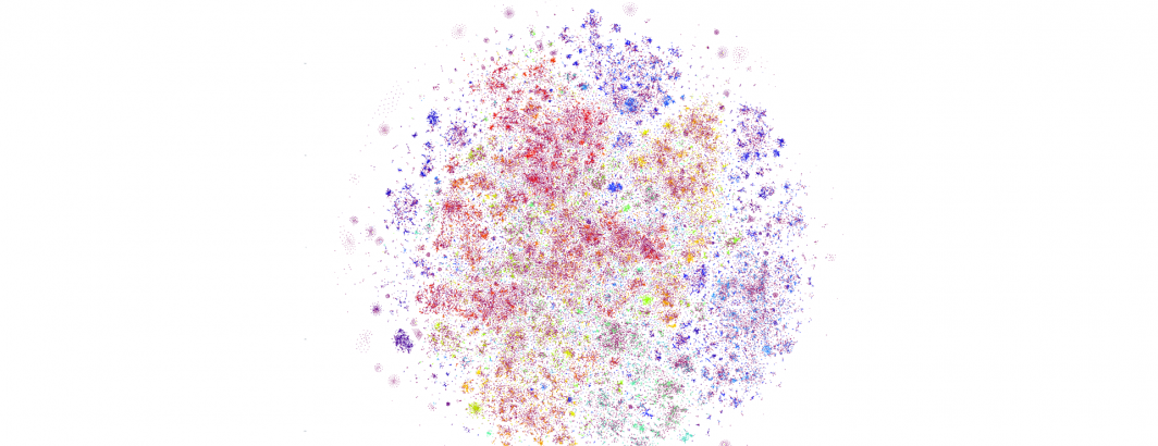
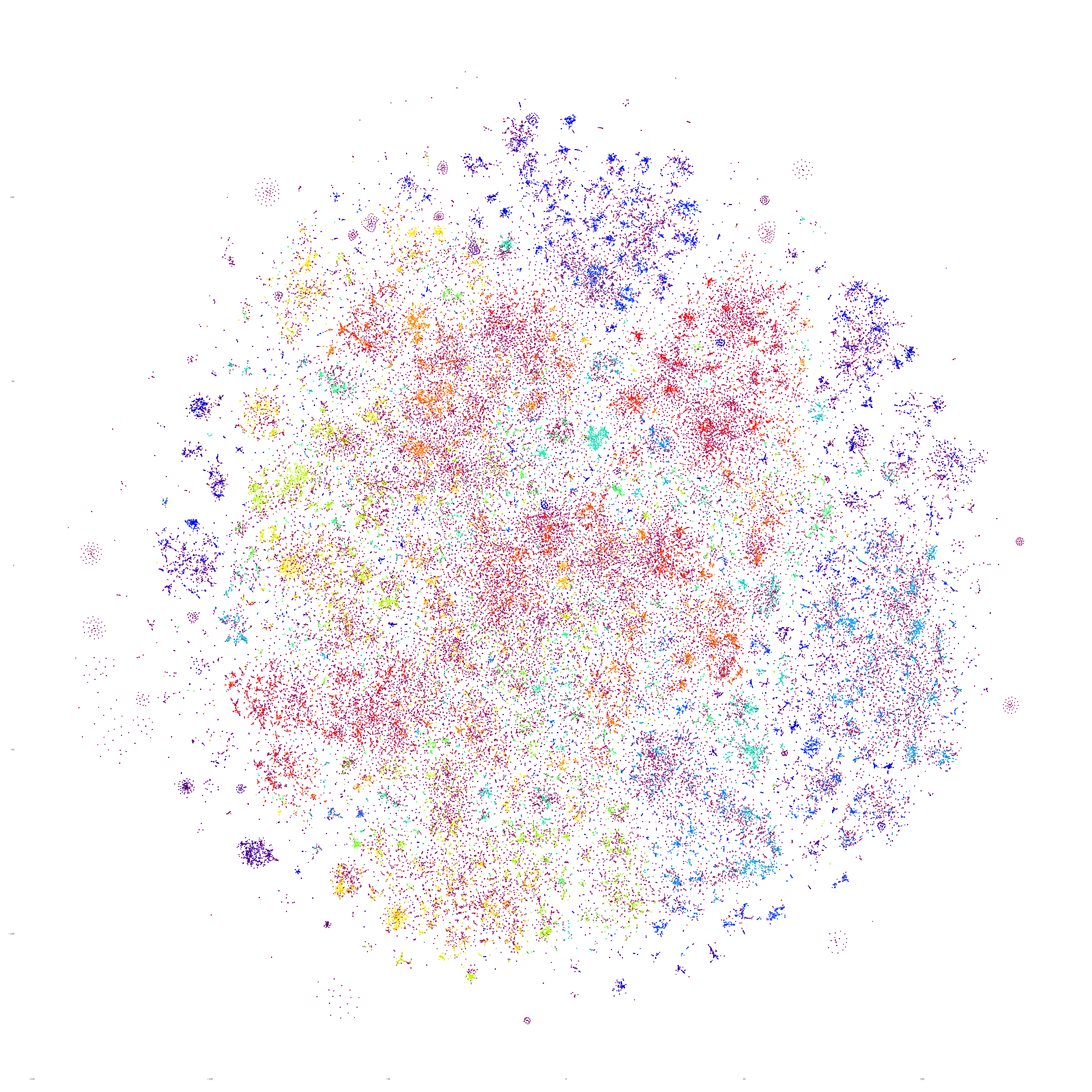
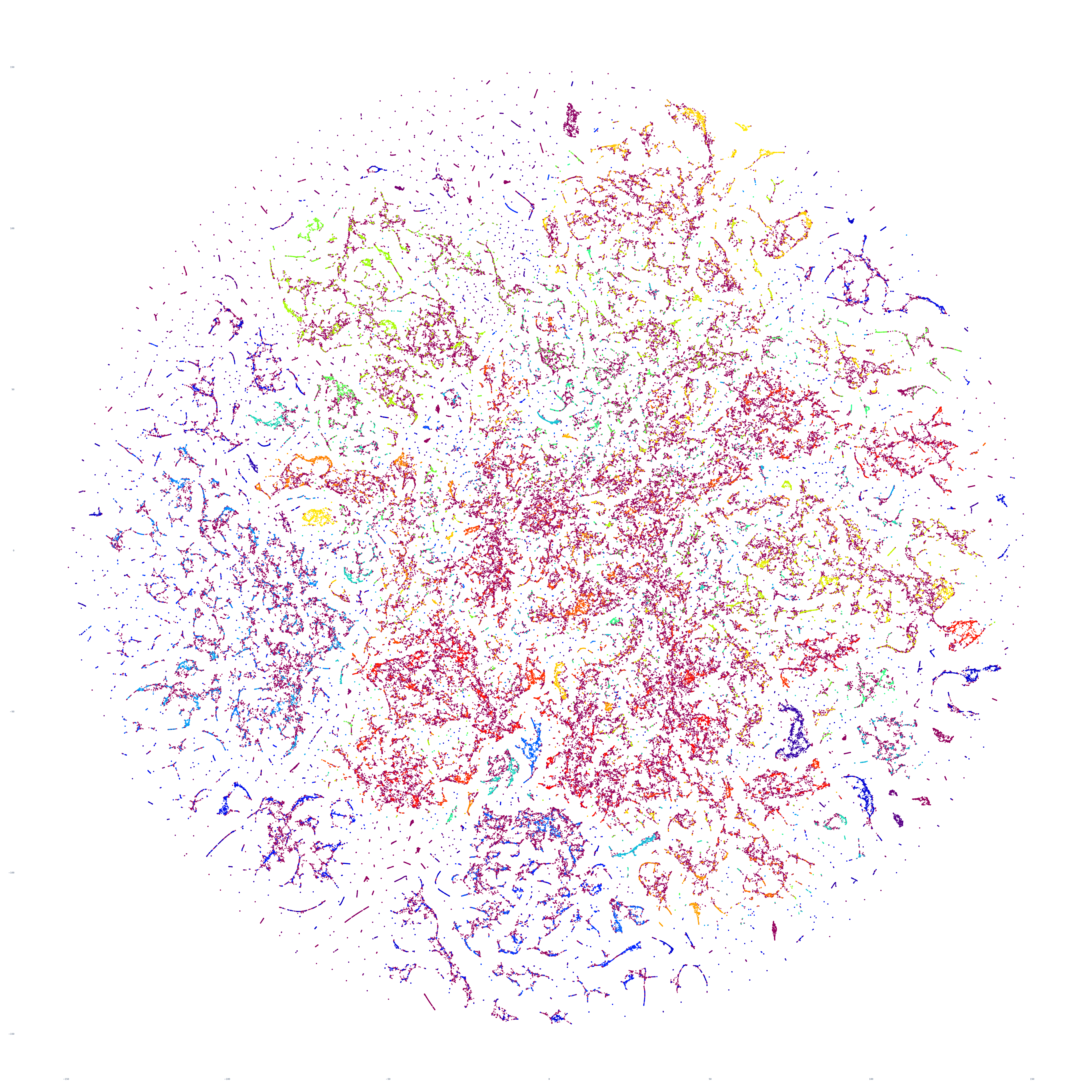
What do the results actually look like? First, let's look at the PCA results. Here is PCA-reduced (to 10 dimensions) HDBSCAN with full resolution t-SNE at 350K articles. The clustering results are largely useless, with nearly the entire dataset reduced to noise (purplish red):
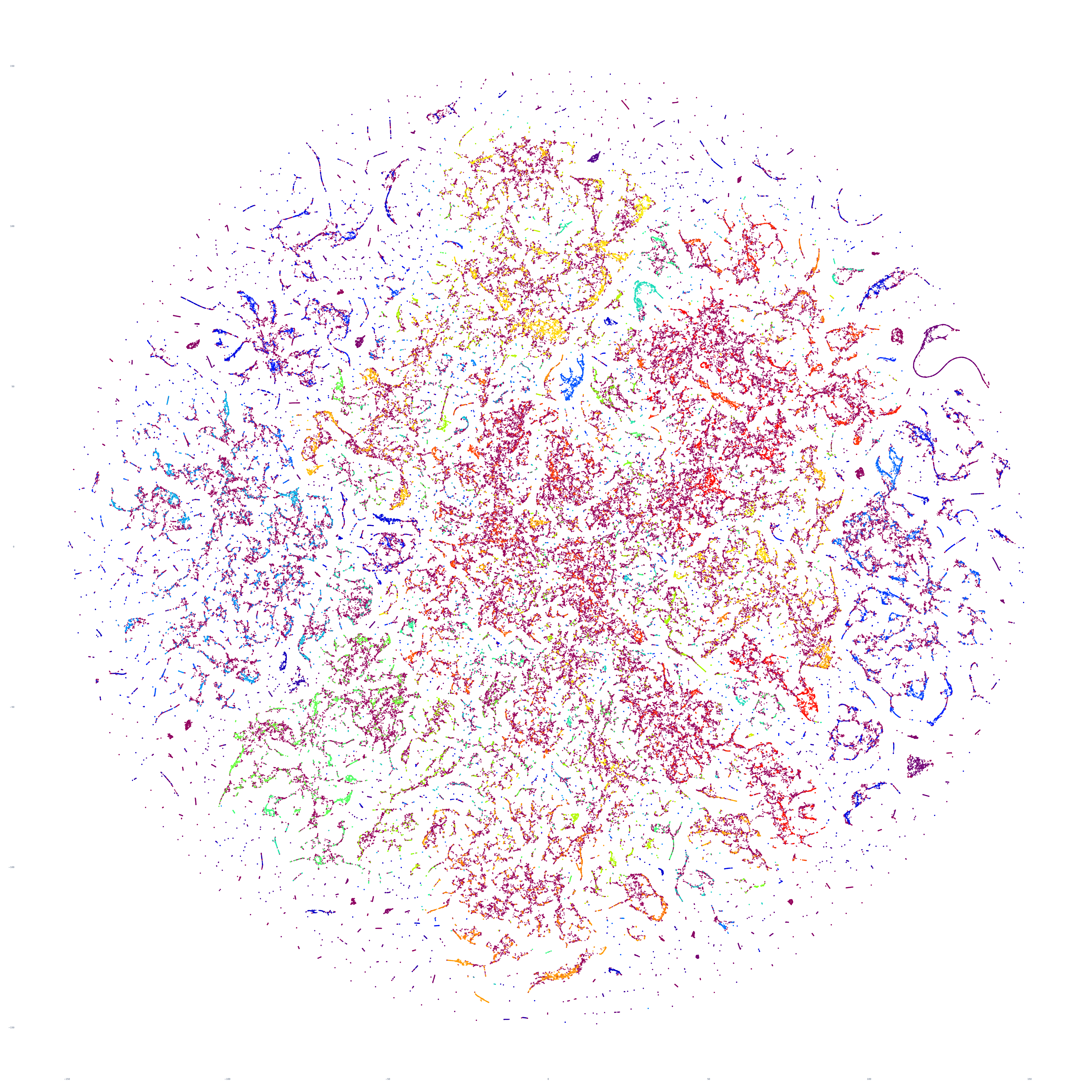
Below is PCA-reduced HDBSCAN with reduced t-SNE. This is effectively useless, with PCA's globalization of the structure preventing t-SNE from performing any form of meaningful structural resolution. Clearly PCA is not a desirable reduction algorithm from the standpoint both of being only marginally faster than UMAP and resulting in terrible results:

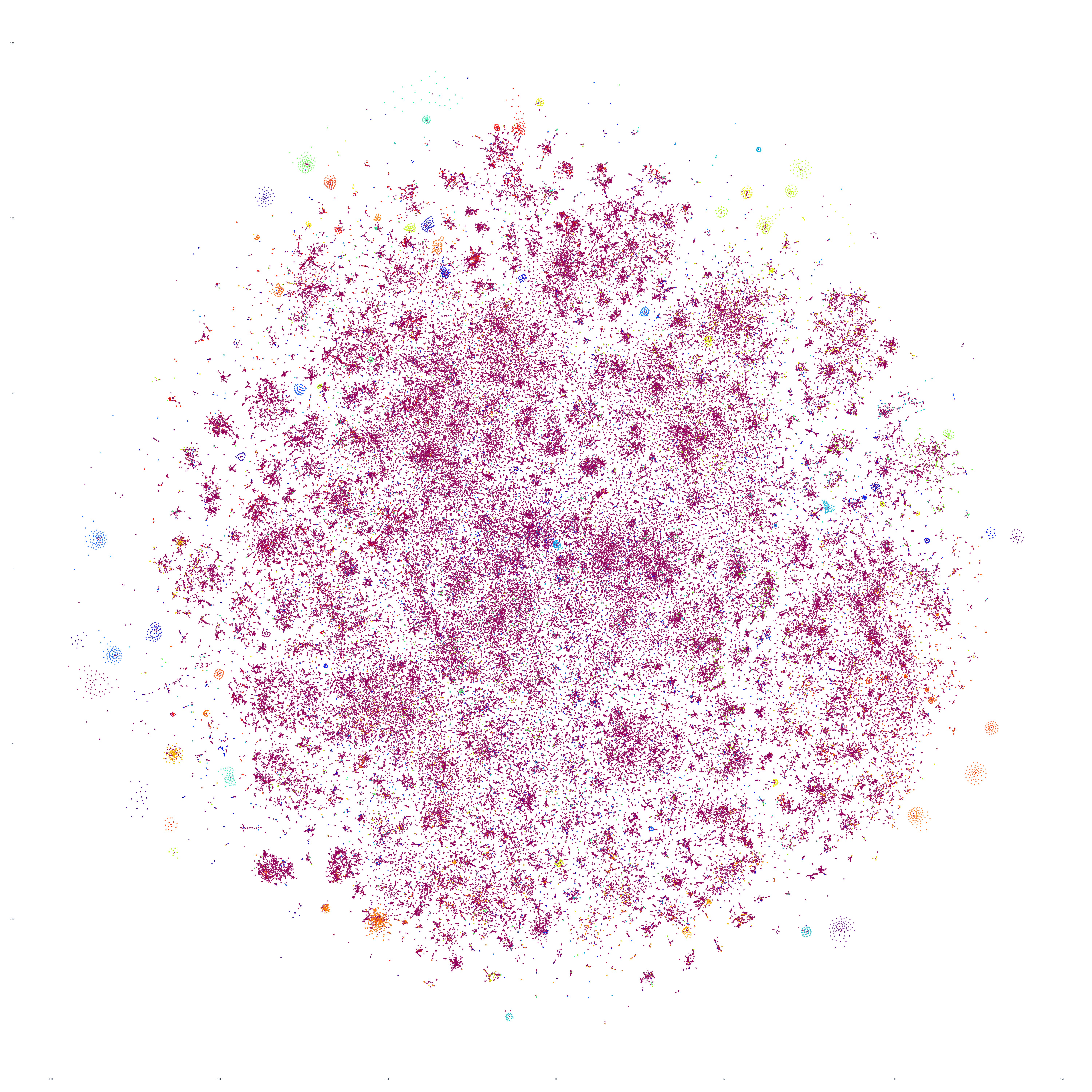
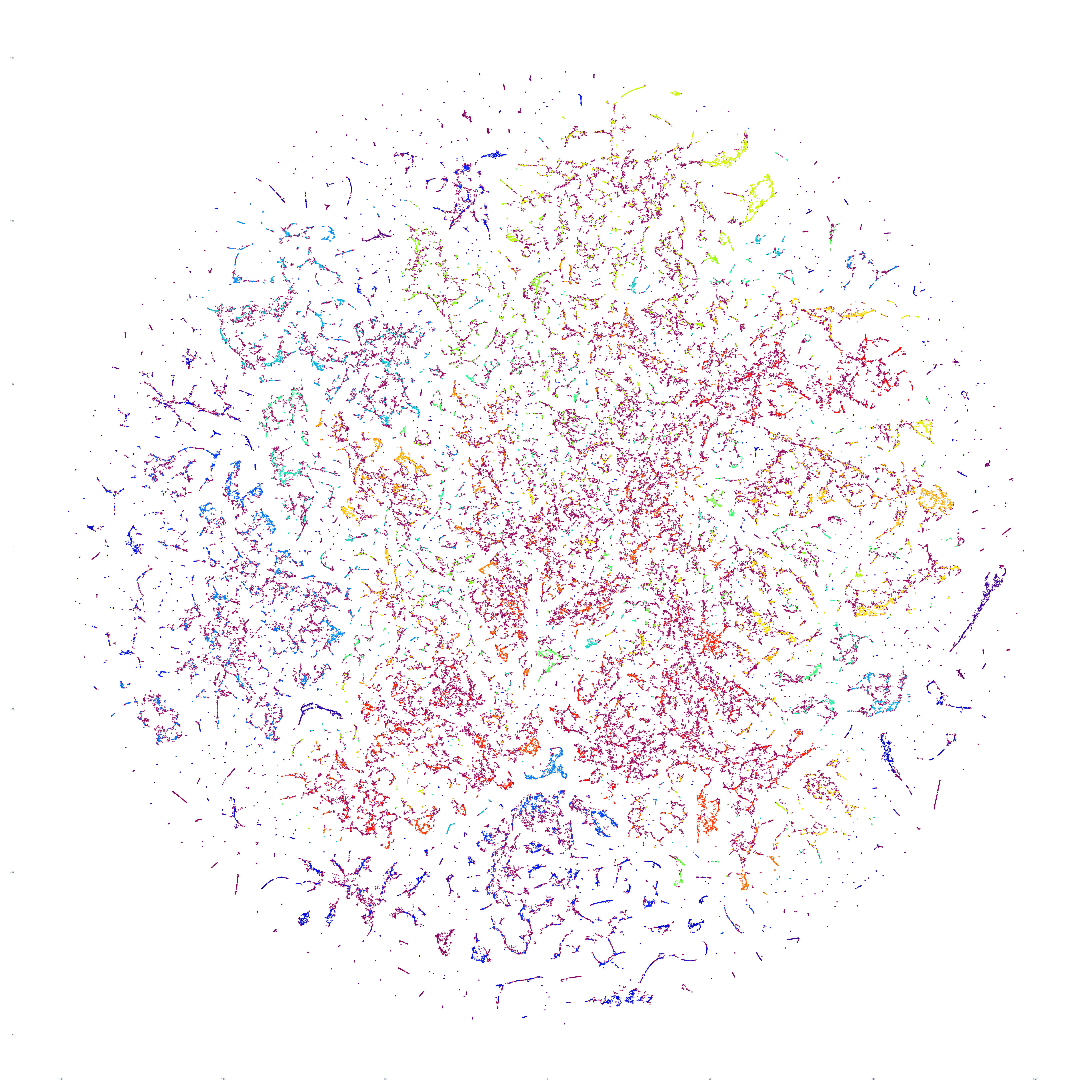
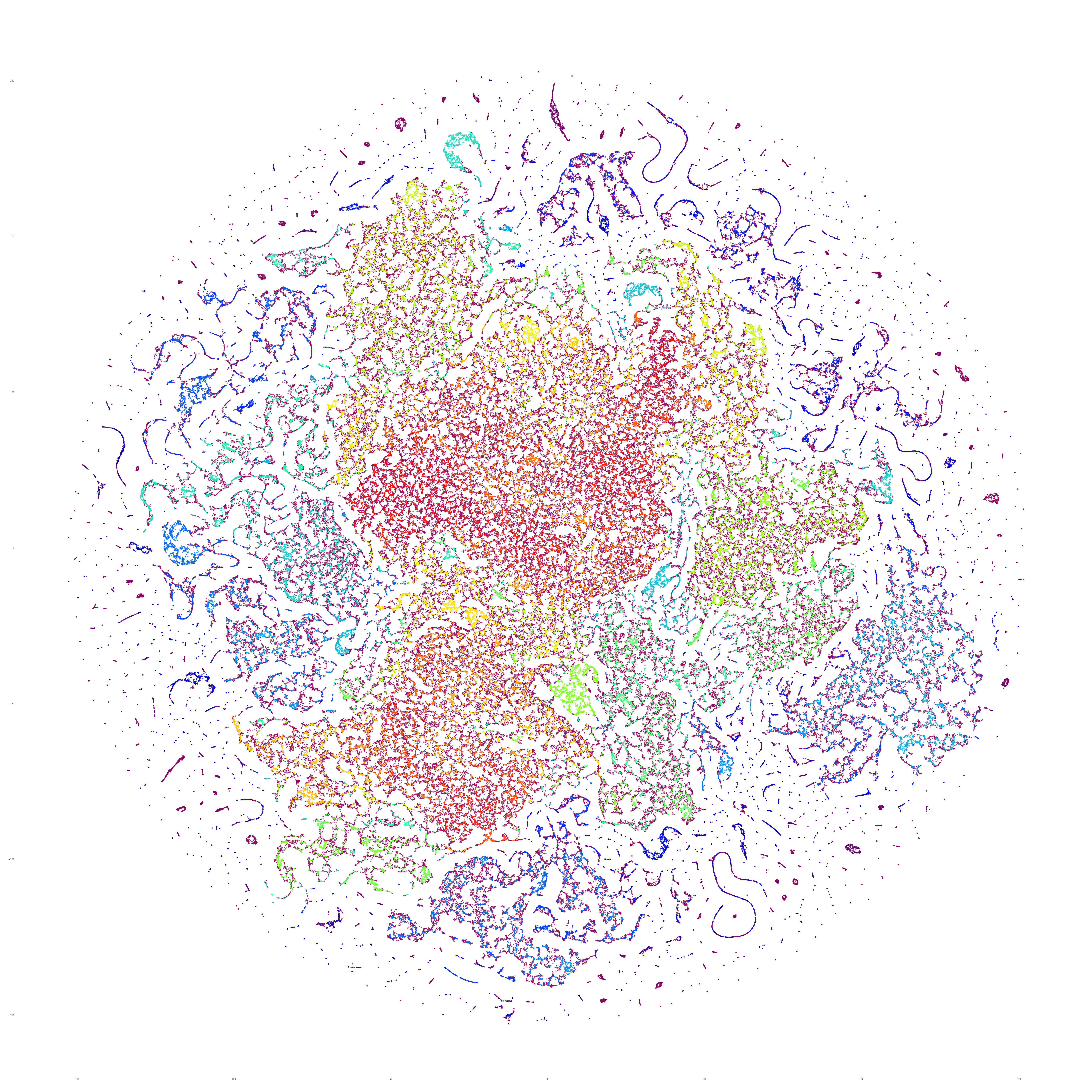
What about the same UMAP reduction for HDBSCAN (to 10 dimensions) and full-resolution (512 dimensions) t-SNE that we used yesterday? For 350K articles, we get exactly what we got yesterday:
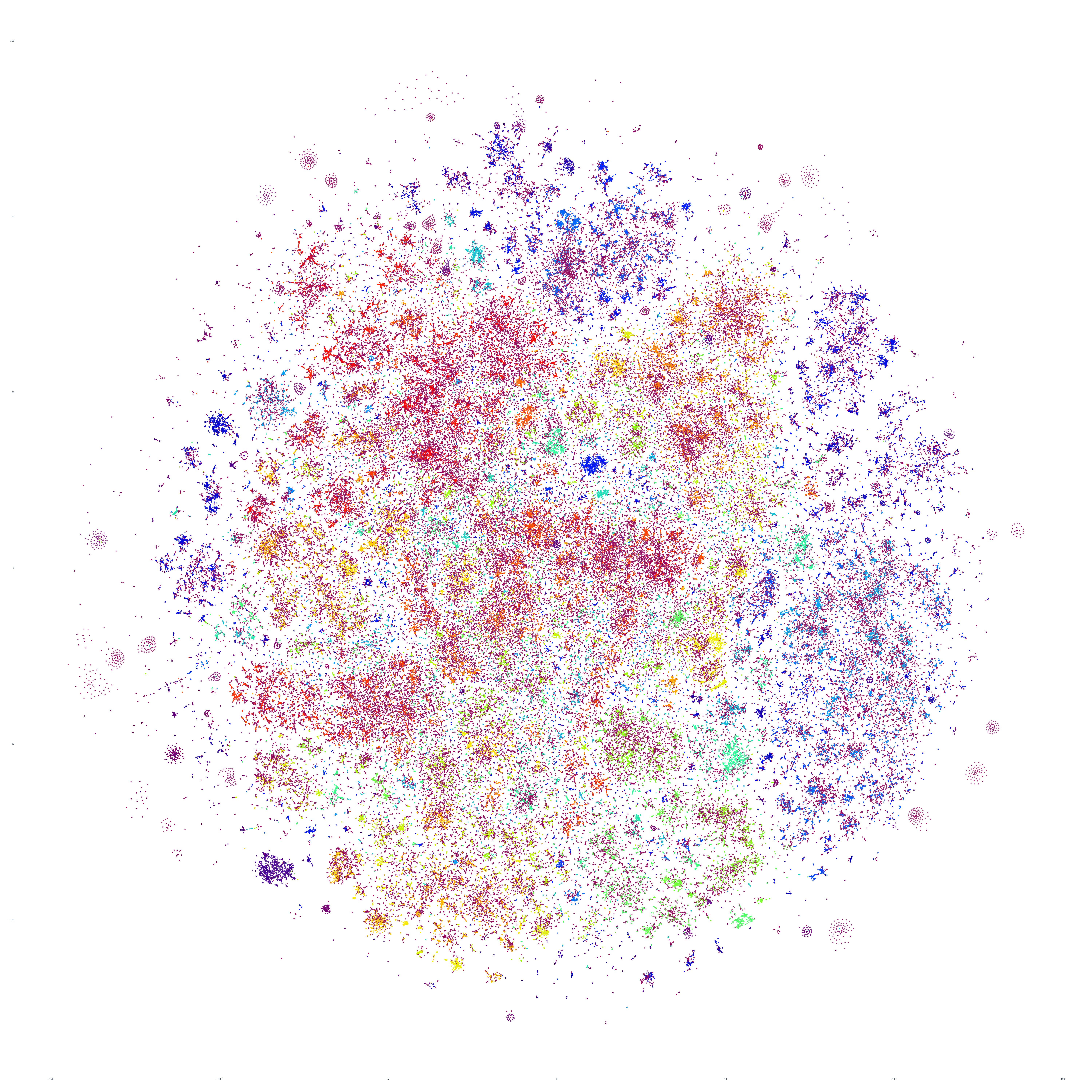
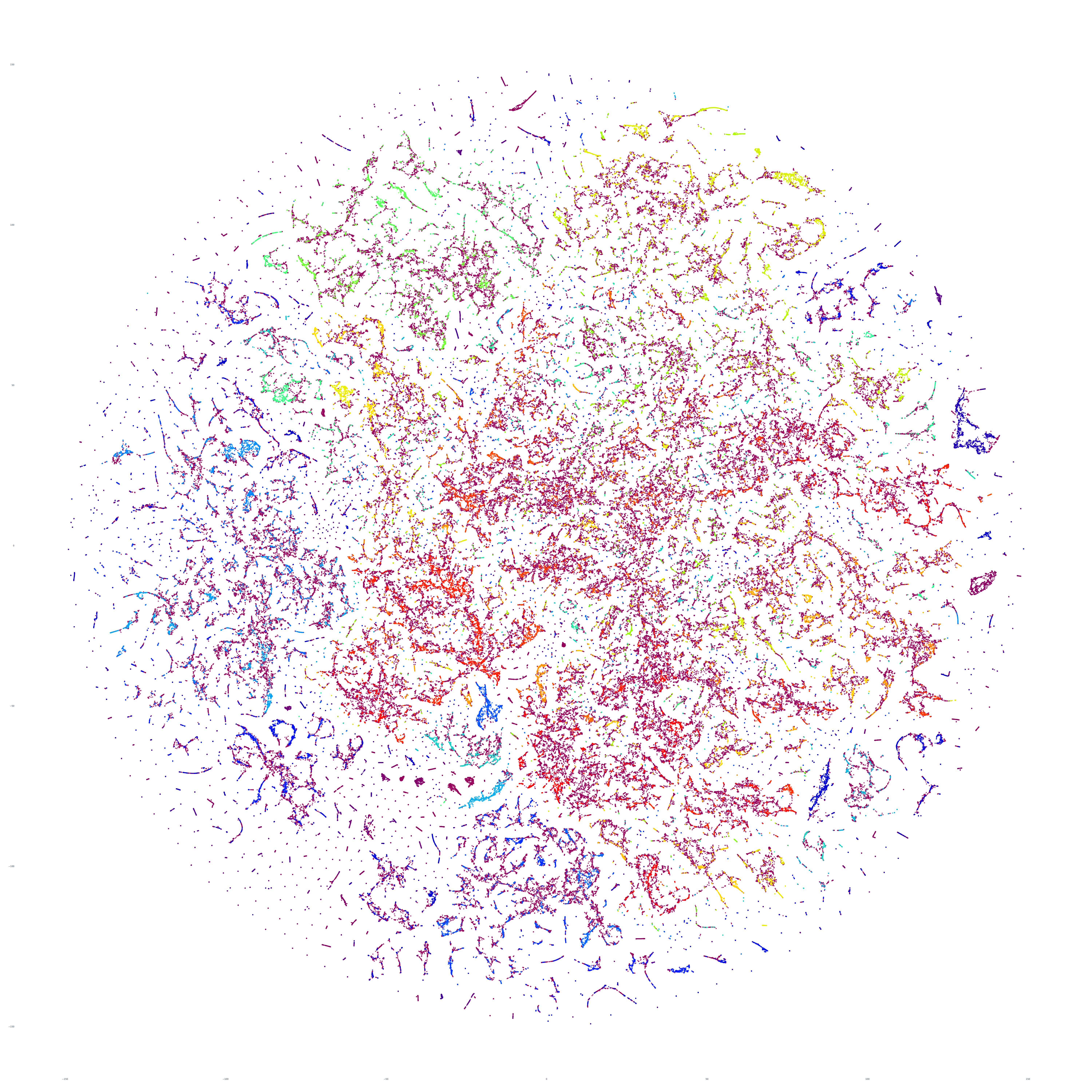
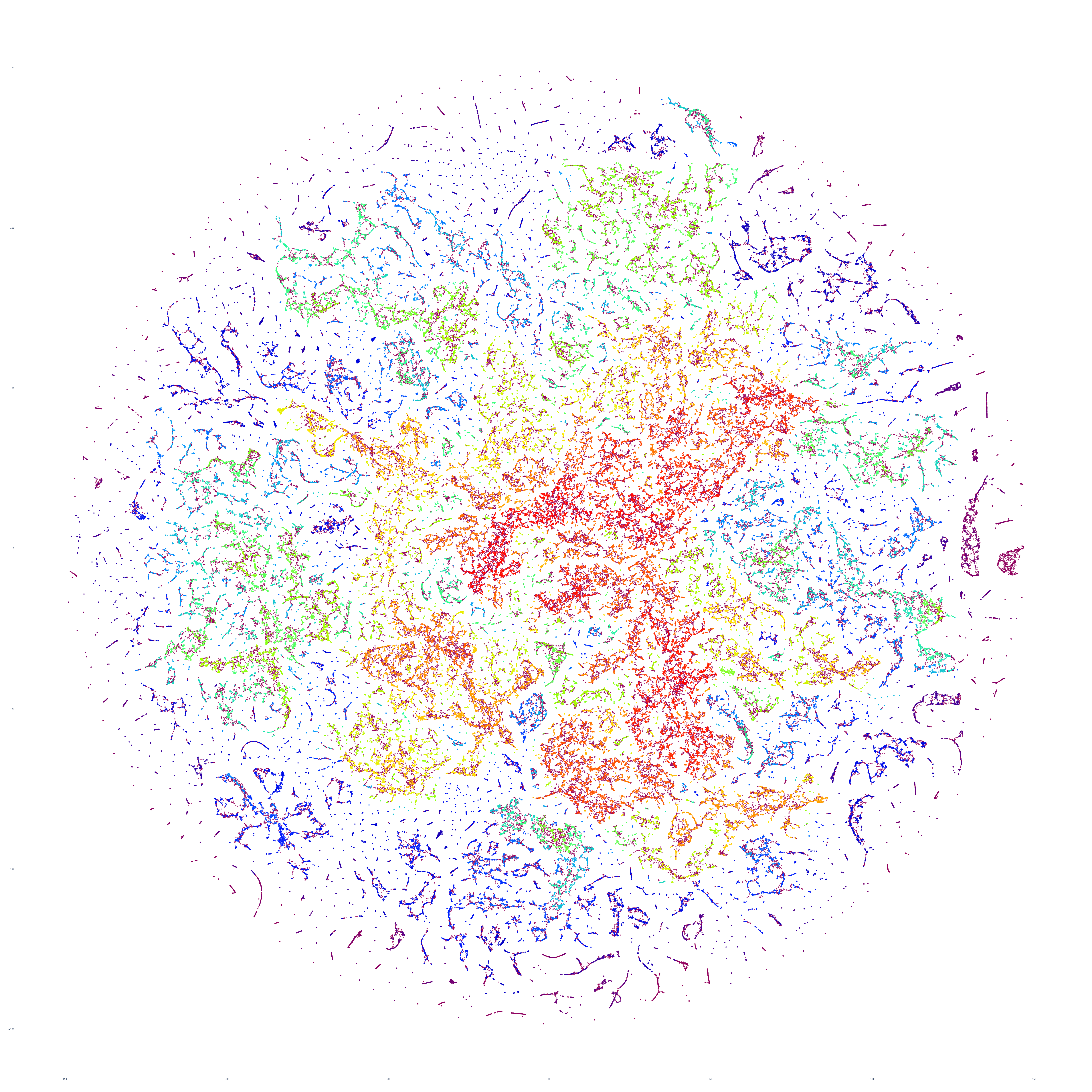
Things get really interesting, however, when we use those same UMAP-reduced embeddings for the t-SNE layout as well. In other words, we use UMAP to reduce our 512-dimension vectors down to 10 dimensions and then use those same reduced 10-dimension vectors for both HDBSCAN clustering and t-SNE layout. All of the diffuse areas above become tendril-like tight interlinked clusters below. This version, while marginally faster, is actually more understandable in many ways, exposing much finer-grained structure. Fascinatingly, the noise articles that form many of the diffuse regions above suddenly become tightly clustered meaningful organizations of articles below.
Looking at the reduced 200K sampled version we can see these results even more clearly. Here is the original UMAP-reduced HDBSCAN + full-resolution t-SNE layout:
And here is the version using the same UMAP-reduced embeddings (10 dimensions) for t-SNE layout, showing just how strongly it clusters the results:
Let's look at the impact of UMAP dimensionality reduction as we sequentially reduce the number of dimensions considered by t-SNE and HDBSCAN. We'll start with using 10 dimensions for HDBSCAN and the full 512-dimension embeddings for t-SNE layout. This yields large diffuse clusters:
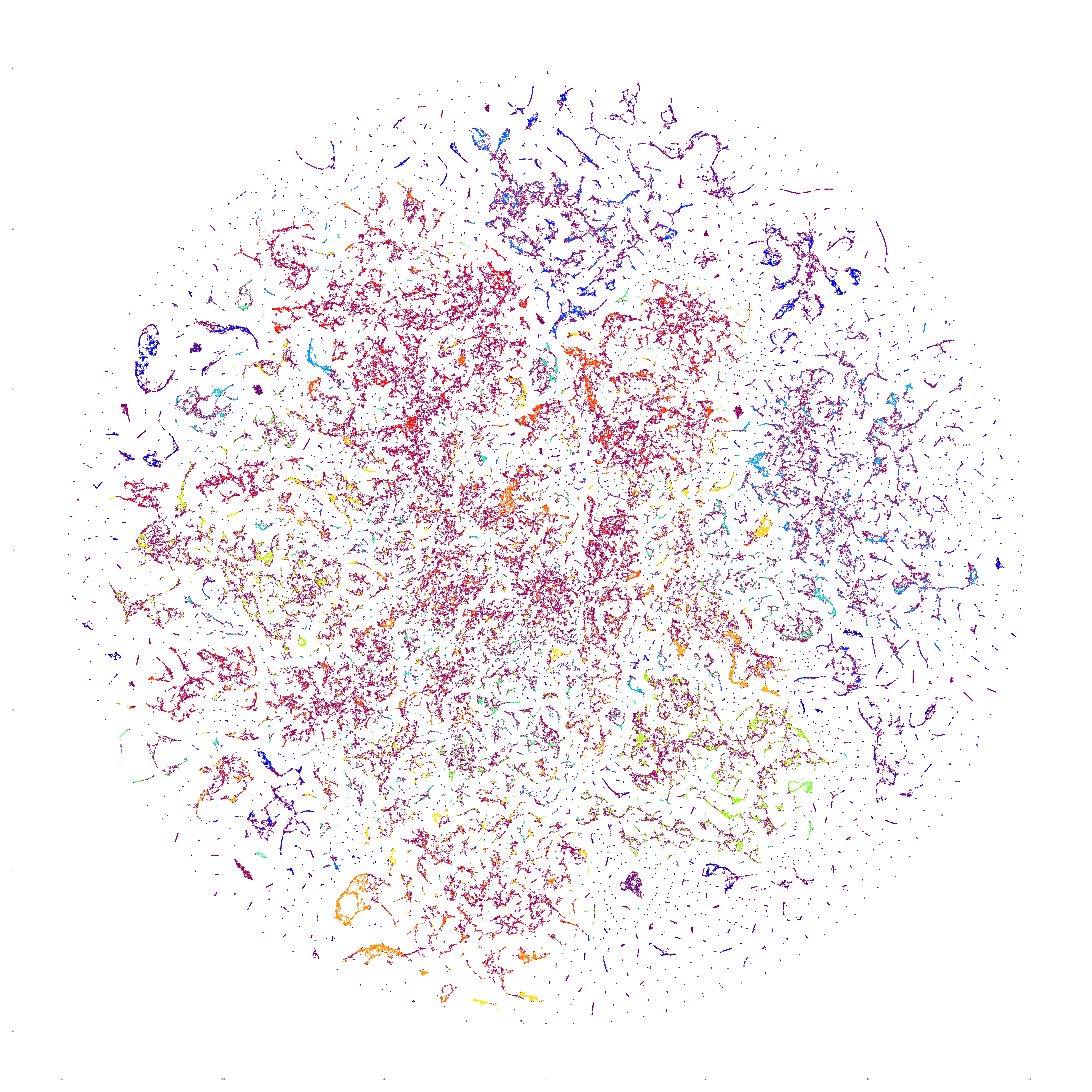
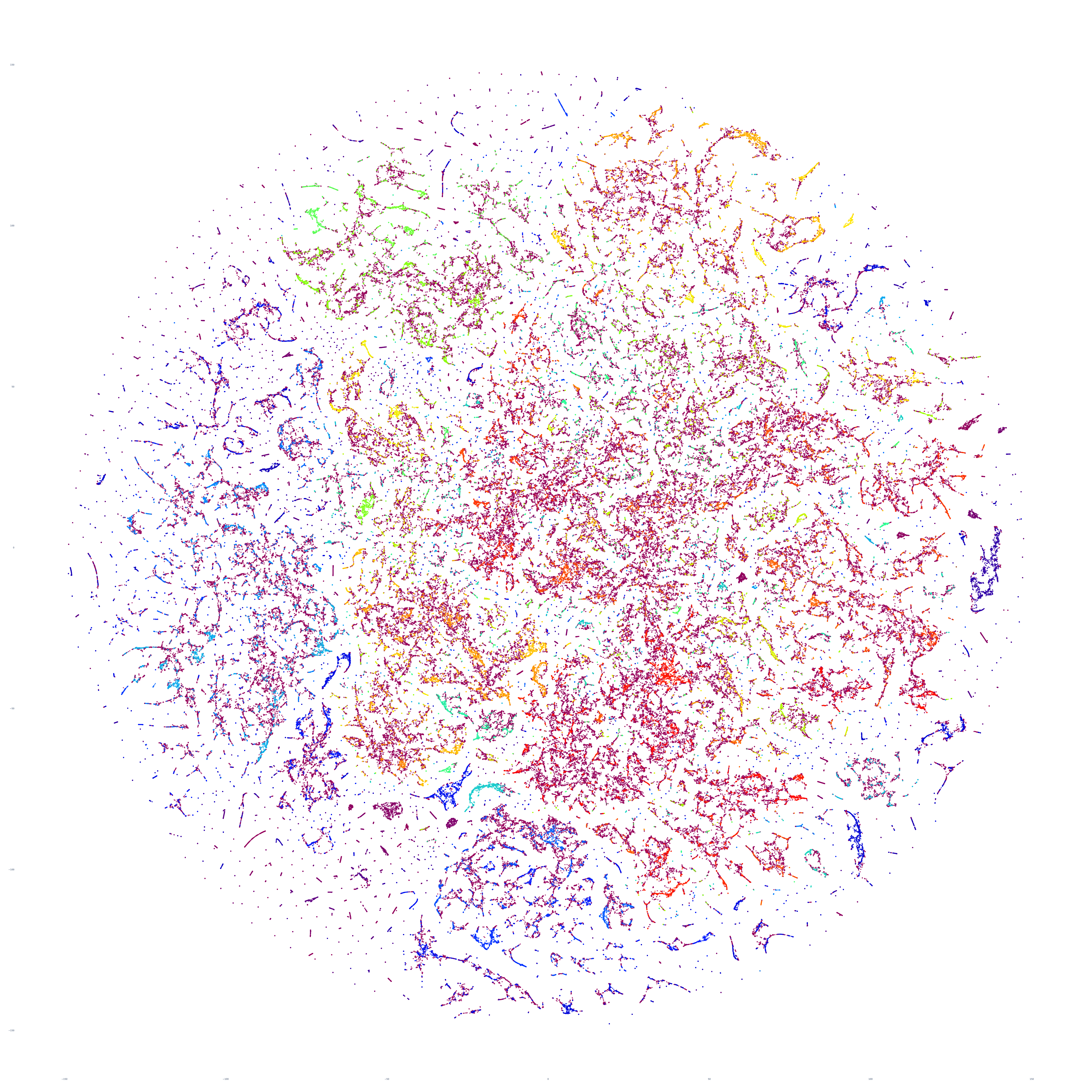
Now we'll use 100 dimensions for both HDBSCAN and t-SNE layout. This results in a drastic change, with the diffuse point clouds that define our full-resolution t-SNE layouts replaced with long interconnected tendrils:
Moving to 50 dimensions for both HDBSCAN and t-SNE layout has only a minimal impact:
Then 25 dimensions for both HDBSCAN and t-SNE layout. This looks nearly identical to 50 dimensions.
Then 10 dimensions for both HDBSCAN and t-SNE layout. Again, few changes.
Then 5 dimensions for both HDBSCAN and t-SNE layout. The results are nearly identical, though perhaps slightly more tendril-like fine structure.
And finally, 2 dimensions for both HDBSCAN and t-SNE layout (with t-SNE then performing 2D layout based on the 2D collapse performed by UMAP). Unlike the previous reductions, which yielded little difference from step to step, this produces a wholesale transformation, organizing the day exclusively into long tendril-like curved structures. Diffuse areas become reorganized into many curved interconnected tendrils. Does this additional structure capture enhanced semantic meaning from the underlying texts, organizing them into meaningful microstructures or does the additional structure actually harm understanding by grouping together unrelated clusters of articles?
Finally, how about our last workflow, where we used UMAP to reduce to 10 dimensions, then t-SNE to collapse to 2D embeddings and used the t-SNE-produced 2D embeddings for both HDBSCAN clustering and visualization? This time we can see much stronger alignment between the coloration and clustering, as HDBSCAN is able to capture the t-SNE-constructed structure, quantifying it into machine-friendly groupings – effectively transforming the visual representation into an machine understandable representation and synchronizing the coloration and layout.
The final Python script used for the analyses here can be found below. Save to "runn.py" and selectively edit accordingly:
#########################
#LOAD THE EMBEDDINGS...

import numpy as np
import matplotlib.pyplot as plt
from PIL import Image
import jsonlines
import multiprocessing
import sys

# Load the JSON file containing embedding vectors
def load_json_embeddings(filename):
    embeddings = []
    titles = []
    langs = []
    with jsonlines.open(filename) as reader:
        for line in reader:
            embeddings.append(line["embed"])
            titles.append(line["title"])
            langs.append(line["lang"])
    return np.array(embeddings), titles, langs

#json_file = 'MASTER.sample.json.500'
json_file = sys.argv[2]
embeddings, titles, langs = load_json_embeddings(json_file)
len(embeddings)

import hdbscan
import umap
from sklearn.decomposition import PCA
import time
clusters = []
embeddings_reduced = []
def cluster_embeddings(embeddings, min_cluster_size=5):
    global clusters, embeddings_reduced
    start_time = time.process_time()
    #embeddings_reduced = PCA(n_components=10, random_state=42).fit_transform(embeddings)
    embeddings_reduced = umap.UMAP(n_neighbors=30,min_dist=0.0,n_components=10,verbose=True).fit_transform(embeddings)
    #embeddings_reduced = umap.UMAP(n_neighbors=30,min_dist=0.0,n_components=5,verbose=True).fit_transform(embeddings)
    end_time = time.process_time()
    elapsed_time = end_time - start_time
    print(f"Dimensionality Reduction: : {elapsed_time} seconds")
    start_time = time.process_time()
    clusterer = hdbscan.HDBSCAN(min_cluster_size=min_cluster_size, core_dist_n_jobs = multiprocessing.cpu_count())
    clusters = clusterer.fit_predict(embeddings_reduced)
    end_time = time.process_time()
    elapsed_time = end_time - start_time
    print(f"HDBSCAN: : {elapsed_time} seconds")
    #return clusters

#cluster...
cluster_embeddings(embeddings, 5)

#output some basic statistics...
unique_clusters = np.unique(clusters)
print("Clusters: " + str(unique_clusters))
print("Num Clusters: " + str(len(unique_clusters)))
cnt_noise = np.count_nonzero(clusters == -1)
print("Noise Articles: " + str(cnt_noise))

#write the output...
with open(sys.argv[1] + '.tsv', 'w', encoding='utf-8') as tsv_file:
    for cluster_id, title, lang in zip(clusters, titles, langs):
        tsv_file.write(f"{cluster_id}\t{title}\t{lang}\n")
print("Wrote Clusters")

#########################
#VISUALIZE...

from sklearn.manifold import TSNE
from sklearn.decomposition import PCA
import plotly.graph_objs as graph
import plotly.io as pio

def plotPointCloud(embeddings, clusters, titles, langs, title, algorithm):
    if (algorithm == 'PCA'):
        start_time = time.process_time()
        pca = PCA(n_components=2, random_state=42)
        embeds = pca.fit_transform(embeddings)
        end_time = time.process_time()
        elapsed_time = end_time - start_time
        print(f"Layout (PCA): {elapsed_time} seconds")
    if (algorithm == 'TSNE'):
        start_time = time.process_time()
        tsne = TSNE(n_components=2, random_state=42)
        embeds = tsne.fit_transform(embeddings)
        #embeds = tsne.fit_transform(embeddings_reduced)
        end_time = time.process_time()
        elapsed_time = end_time - start_time
        print(f"Layout (TSNE): {elapsed_time} seconds")

    start_time = time.process_time()
    trace = graph.Scatter(
        x=embeds[:, 0],
        y=embeds[:, 1],
        marker=dict(
            size=6,
            #color=np.arange(len(embeds)), #color randomly
            color=clusters, #color via HDBSCAN clusters
            colorscale='Rainbow',
            opacity=0.8
        ),
        #text = langs,
        #text = titles,
        #text = [title[:20] for title in titles],
        hoverinfo='text',
        #mode='markers+text',
        mode='markers',
        textposition='bottom right'
    )

    layout = graph.Layout(
        #title=title,
        xaxis=dict(title=''),
        yaxis=dict(title=''),
        height=6000,
        width=6000,
        plot_bgcolor='rgba(255,255,255,255)',
        hovermode='closest',
        hoverlabel=dict(bgcolor="black", font_size=14)
    )

    fig = graph.Figure(data=[trace], layout=layout)
    fig.update_layout(autosize=True)

    # Save the figure as a PNG image
    pio.write_image(fig, sys.argv[1] + '.png', format='png')
    end_time = time.process_time()
    elapsed_time = end_time - start_time
    print(f"Render: {elapsed_time} seconds")

# Call the function with your data
#clusters = []
plotPointCloud(embeddings, clusters, titles, langs, 'Title', 'TSNE')
#########################
For those interested in downloading the underlying TSV files for further analysis to see how various methods split the groupings different ways, you can download them via the URLs below:
https://storage.googleapis.com/data.gdeltproject.org/blog/2023-atscaleembeddingclusteringexperiments/output-100k-pcahdbscan-tsnareduced10.tsv
https://storage.googleapis.com/data.gdeltproject.org/blog/2023-atscaleembeddingclusteringexperiments/output-100k-tsnafull.tsv
https://storage.googleapis.com/data.gdeltproject.org/blog/2023-atscaleembeddingclusteringexperiments/output-100k-umap5hdbscan-tsnafull.tsv
https://storage.googleapis.com/data.gdeltproject.org/blog/2023-atscaleembeddingclusteringexperiments/output-100k-umap5hdbscan-tsnareduced5.tsv
https://storage.googleapis.com/data.gdeltproject.org/blog/2023-atscaleembeddingclusteringexperiments/output-100k-umaphdbscan-tsnafull.tsv
https://storage.googleapis.com/data.gdeltproject.org/blog/2023-atscaleembeddingclusteringexperiments/output-100k-umaphdbscan-tsnareduced10.tsv
https://storage.googleapis.com/data.gdeltproject.org/blog/2023-atscaleembeddingclusteringexperiments/output-10k-pcahdbscan-tsnafull.tsv
https://storage.googleapis.com/data.gdeltproject.org/blog/2023-atscaleembeddingclusteringexperiments/output-10k-pcahdbscan-tsnareduced10.tsv
https://storage.googleapis.com/data.gdeltproject.org/blog/2023-atscaleembeddingclusteringexperiments/output-10k-umap5hdbscan-tsnafull.tsv
https://storage.googleapis.com/data.gdeltproject.org/blog/2023-atscaleembeddingclusteringexperiments/output-10k-umap5hdbscan-tsnareduced5.tsv
https://storage.googleapis.com/data.gdeltproject.org/blog/2023-atscaleembeddingclusteringexperiments/output-10k-umaphdbscan-tsnafull.tsv
https://storage.googleapis.com/data.gdeltproject.org/blog/2023-atscaleembeddingclusteringexperiments/output-10k-umaphdbscan-tsnareduced10.tsv
https://storage.googleapis.com/data.gdeltproject.org/blog/2023-atscaleembeddingclusteringexperiments/output-200k-pcahdbscan-tsnafull.tsv
https://storage.googleapis.com/data.gdeltproject.org/blog/2023-atscaleembeddingclusteringexperiments/output-200k-pcahdbscan-tsnareduced10.tsv
https://storage.googleapis.com/data.gdeltproject.org/blog/2023-atscaleembeddingclusteringexperiments/output-200k-umap5hdbscan-tsnafull.tsv
https://storage.googleapis.com/data.gdeltproject.org/blog/2023-atscaleembeddingclusteringexperiments/output-200k-umap5hdbscan-tsnareduced5.tsv
https://storage.googleapis.com/data.gdeltproject.org/blog/2023-atscaleembeddingclusteringexperiments/output-200k-umaphdbscan-tsnafull.tsv
https://storage.googleapis.com/data.gdeltproject.org/blog/2023-atscaleembeddingclusteringexperiments/output-200k-umaphdbscan-tsnareduced10.tsv
https://storage.googleapis.com/data.gdeltproject.org/blog/2023-atscaleembeddingclusteringexperiments/output-350k-pcahdbscan-tsnafull.tsv
https://storage.googleapis.com/data.gdeltproject.org/blog/2023-atscaleembeddingclusteringexperiments/output-350k-pcahdbscan-tsnareduced10.tsv
https://storage.googleapis.com/data.gdeltproject.org/blog/2023-atscaleembeddingclusteringexperiments/output-350k-umap100hdbscan-tsnareduced100.tsv
https://storage.googleapis.com/data.gdeltproject.org/blog/2023-atscaleembeddingclusteringexperiments/output-350k-umap25hdbscan-tsnareduced25.tsv
https://storage.googleapis.com/data.gdeltproject.org/blog/2023-atscaleembeddingclusteringexperiments/output-350k-umap2hdbscan-tsnareduced2.tsv
https://storage.googleapis.com/data.gdeltproject.org/blog/2023-atscaleembeddingclusteringexperiments/output-350k-umap50hdbscan-tsnareduced50.tsv
https://storage.googleapis.com/data.gdeltproject.org/blog/2023-atscaleembeddingclusteringexperiments/output-350k-umap5hdbscan-tsnafull.tsv
https://storage.googleapis.com/data.gdeltproject.org/blog/2023-atscaleembeddingclusteringexperiments/output-350k-umap5hdbscan-tsnareduced5.tsv
https://storage.googleapis.com/data.gdeltproject.org/blog/2023-atscaleembeddingclusteringexperiments/output-350k-umaphdbscan-tsnafull.tsv
https://storage.googleapis.com/data.gdeltproject.org/blog/2023-atscaleembeddingclusteringexperiments/output-350k-umaphdbscan-tsnareduced10.tsv
https://storage.googleapis.com/data.gdeltproject.org/blog/2023-atscaleembeddingclusteringexperiments/output-350k-umaptosne10hdbscan-tsnareduced10paired.tsv
https://storage.googleapis.com/data.gdeltproject.org/blog/2023-atscaleembeddingclusteringexperiments/output-500-pcahdbscan-tsnafull.tsv
https://storage.googleapis.com/data.gdeltproject.org/blog/2023-atscaleembeddingclusteringexperiments/output-500-pcahdbscan-tsnareduced10.tsv
https://storage.googleapis.com/data.gdeltproject.org/blog/2023-atscaleembeddingclusteringexperiments/output-500-umap5hdbscan-tsnafull.tsv
https://storage.googleapis.com/data.gdeltproject.org/blog/2023-atscaleembeddingclusteringexperiments/output-500-umap5hdbscan-tsnareduced5.tsv
https://storage.googleapis.com/data.gdeltproject.org/blog/2023-atscaleembeddingclusteringexperiments/output-500-umaphdbscan-tsnafull.tsv
https://storage.googleapis.com/data.gdeltproject.org/blog/2023-atscaleembeddingclusteringexperiments/output-500-umaphdbscan-tsnareduced10.tsv