Last week we visualized an entire day of television news coverage through the eyes of three channels in China, Iran and Russia, demonstrating the incredible power of at-scale exploration of the global media landscape. What would it look like to scale this concept all the way up to visualize an entire day of global news coverage encompassing all of the countries GDELT monitors? To create quite literally a map of planet earth on a single day?
The end result is that there is a certain level of uniformity to the daily news landscape in terms of macro-level structure, with the world's nations, cultures and citizenry forming a predictable tapestry of coverage each day, with the biggest international stories influencing that fabric sufficiently on a week-by-week basis to be visible in the greater uniformity of its structure. There are many unknowns about the graphs below, including the degree to which the underlying embedding model (USEv4), choice of fulltext embedding (vs title, lede or other surrogates), clustering (HDBSCAN), layout (t-SNE), tractability enhancements (UMAP-based dimensionality-reduction) or other aspects of this workflow may influence these results and we will be exploring these dimensions in additional experiments to come.
To take the first steps towards this vision we'll use the Global Similarity Graph Document Embeddings (GSG) dataset, which covers the 65 languages GDELT 2.0 live-translates, offering 512-dimension embeddings for each article through the Universal Sentence Encoder V4. Uniquely, the GSG leverages USEv4's DAN-based architecture to construct embeddings over the complete machine translated fulltext of each article, meaning the embeddings represent the complete coverage of each article, rather than the headline or lede-only embeddings that are more typically used.
We'll use the same day as our television examples (October 17, 2023 UTC). Given the computational intensiveness of some of the clustering and visualization methods here, we'll use a random sample of the full GSG dataset for that day to make our results more tractable and to overcome some scalability limitations and unexpected issues with some of the Python modules we'll be using.
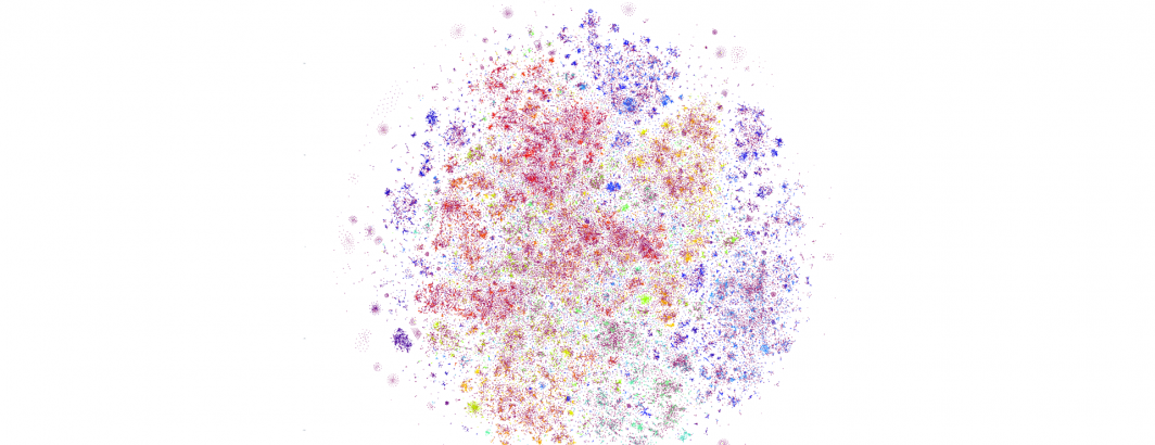
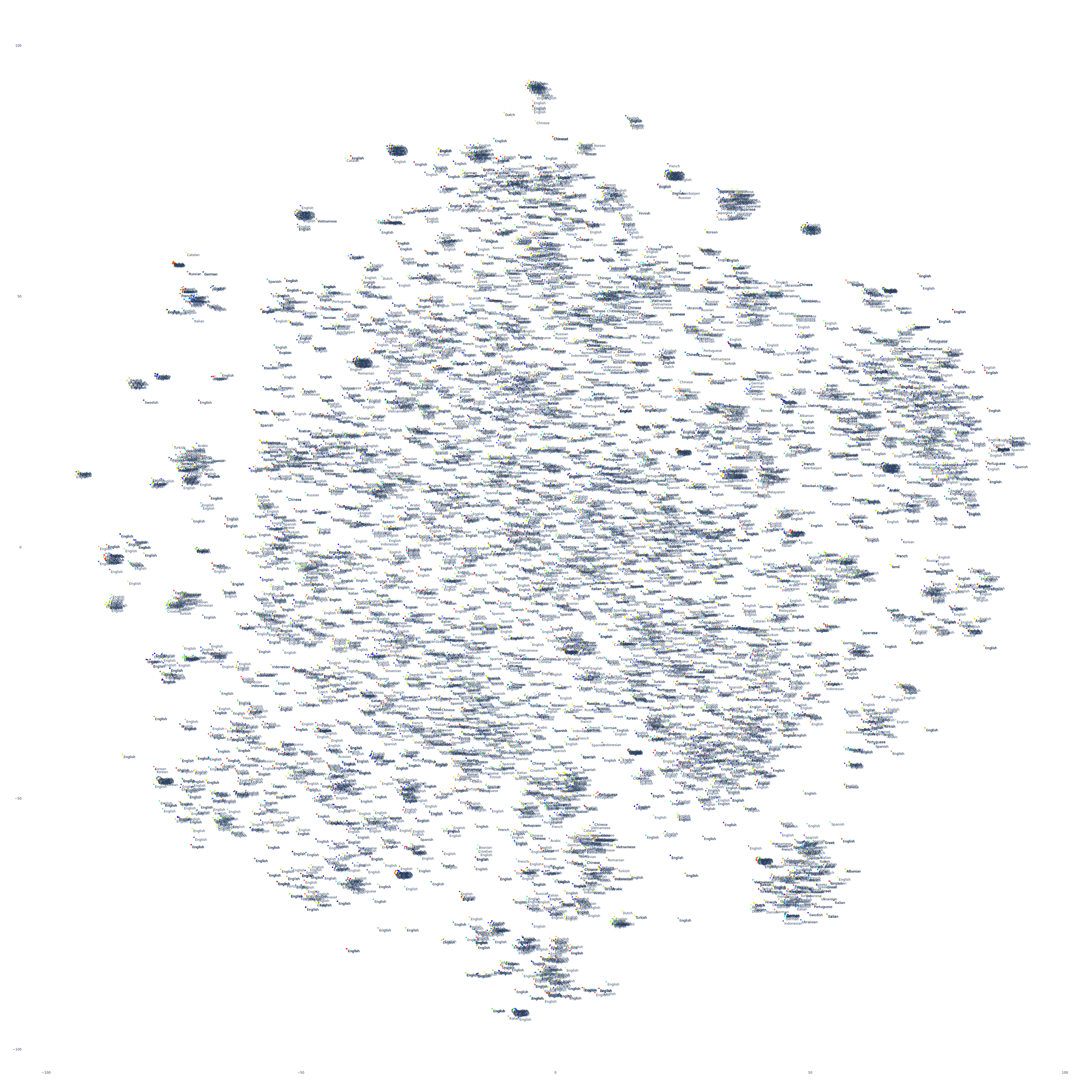
Let's start by visualizing a small random sample of 10,000 articles and their publication languages. Articles that appear closer together are more similar in their contents. We'll use t-SNE for layout. Unsurprisingly, there is a fair degree of linguistic affinity, where stories tend to be covered by a single dominate language due to limited international interest, but look closer and you'll see just how prevalent multilingual clusters are – especially the presence of at least one English article in each cluster, reflecting the dominance of the English language in global news production and coverage.
Let's scale this up to a random sample of 350,000 articles. Unfortunately, we encountered instability issues with the Python library we used to generate the visualizations when attempting to scale past this point, so we'll limit ourselves to that upper bound for this initial experiment. Similar to the image above, each article is represented by a single dot and clustered based on how similar articles are to each other. To make the spatial layout of the clustering more apparent we colored each point effectively at random, so the color of each point below is not meaningful.
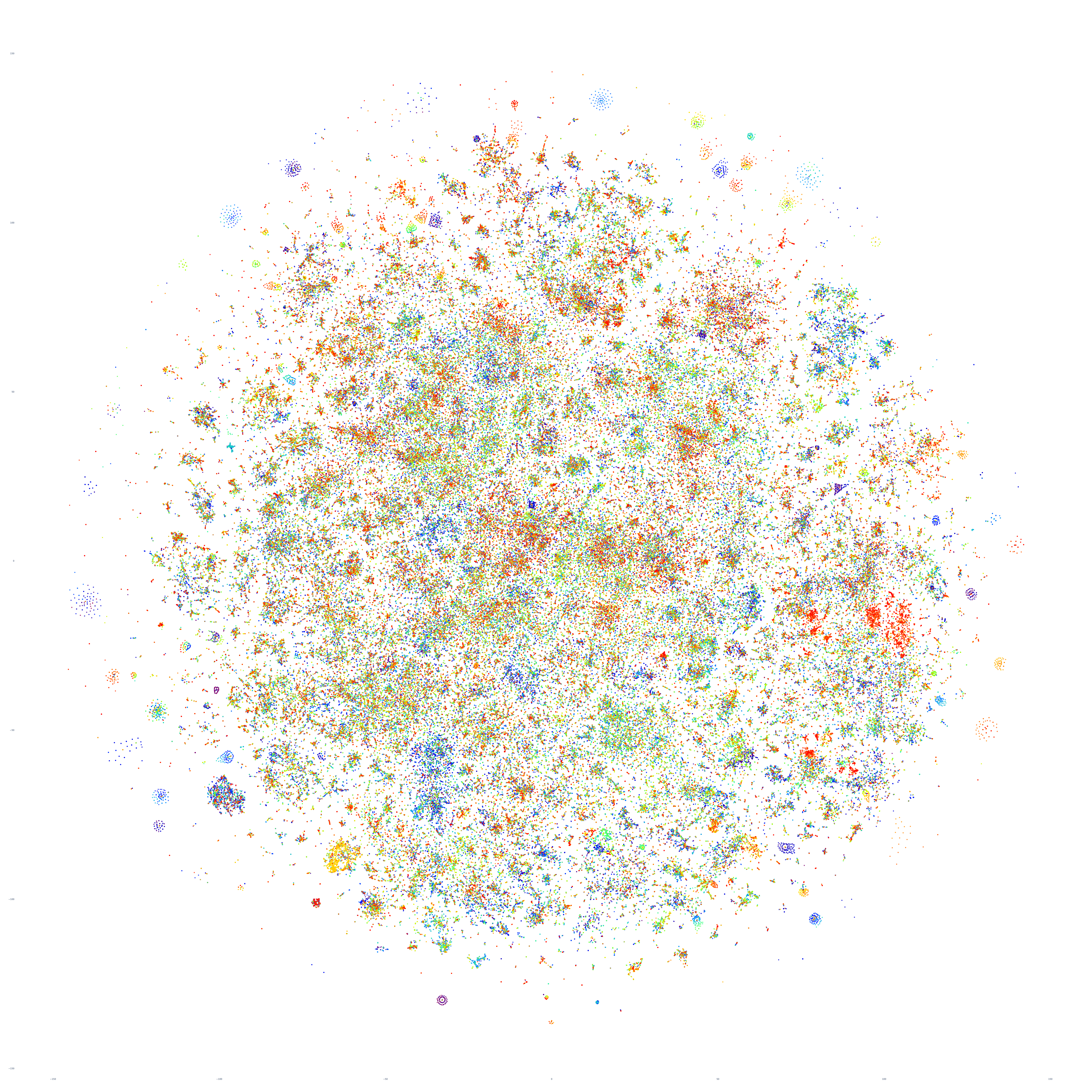
What does this image tell us? Perhaps most powerfully, it tells us that despite several major global-scale stories dominating American media on October 17th, when we look at the planetary-scale media landscape, we see a vast diffuse landscape of countless multiscale clusters – a diffuse cloud of points with innate structure but no major centrality. In other words, Planet Earth on October 17th was defined not by a handful of major stories eclipsing all else, but rather myriad stories from every corner of the globe capturing the heartbeat of the planet we call home.
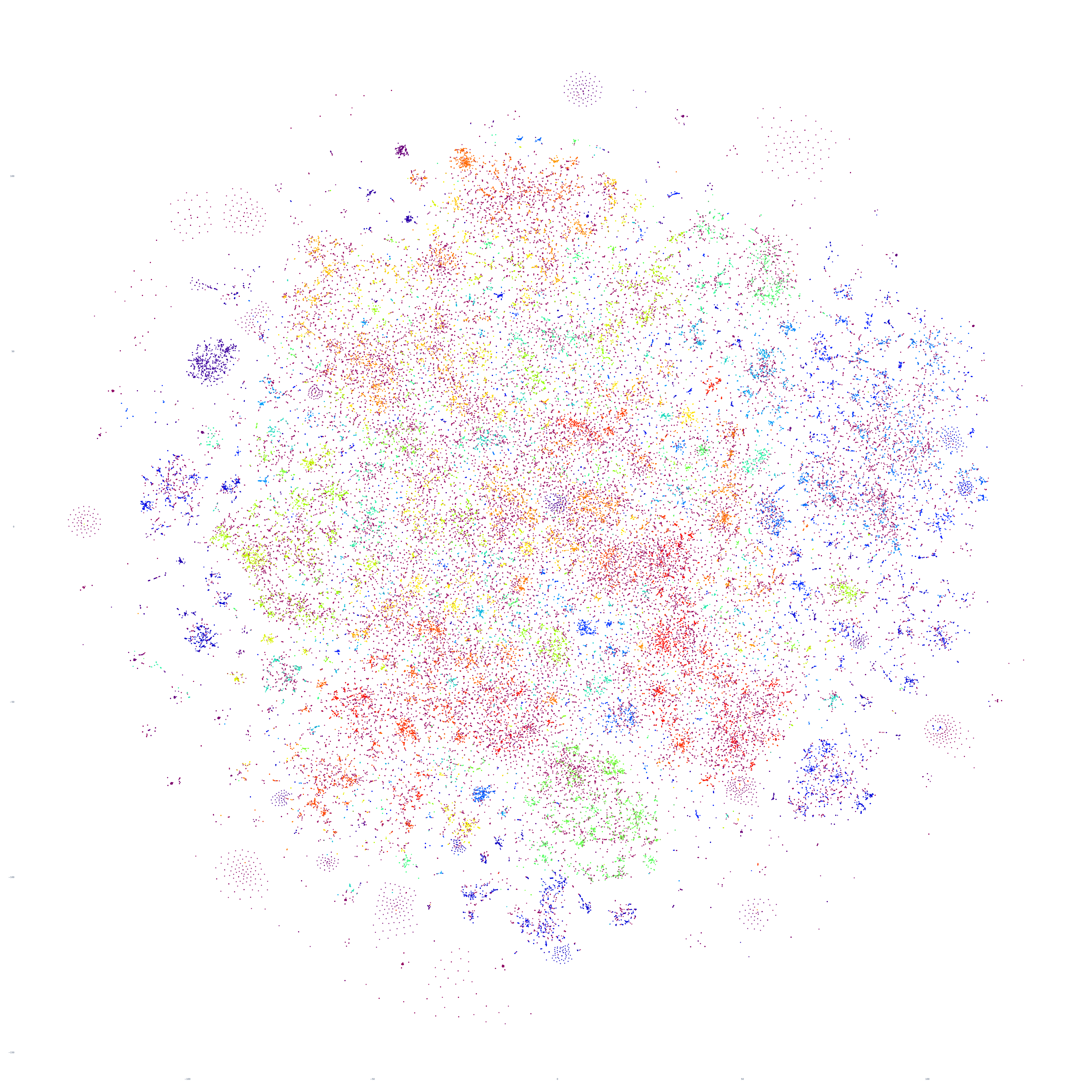
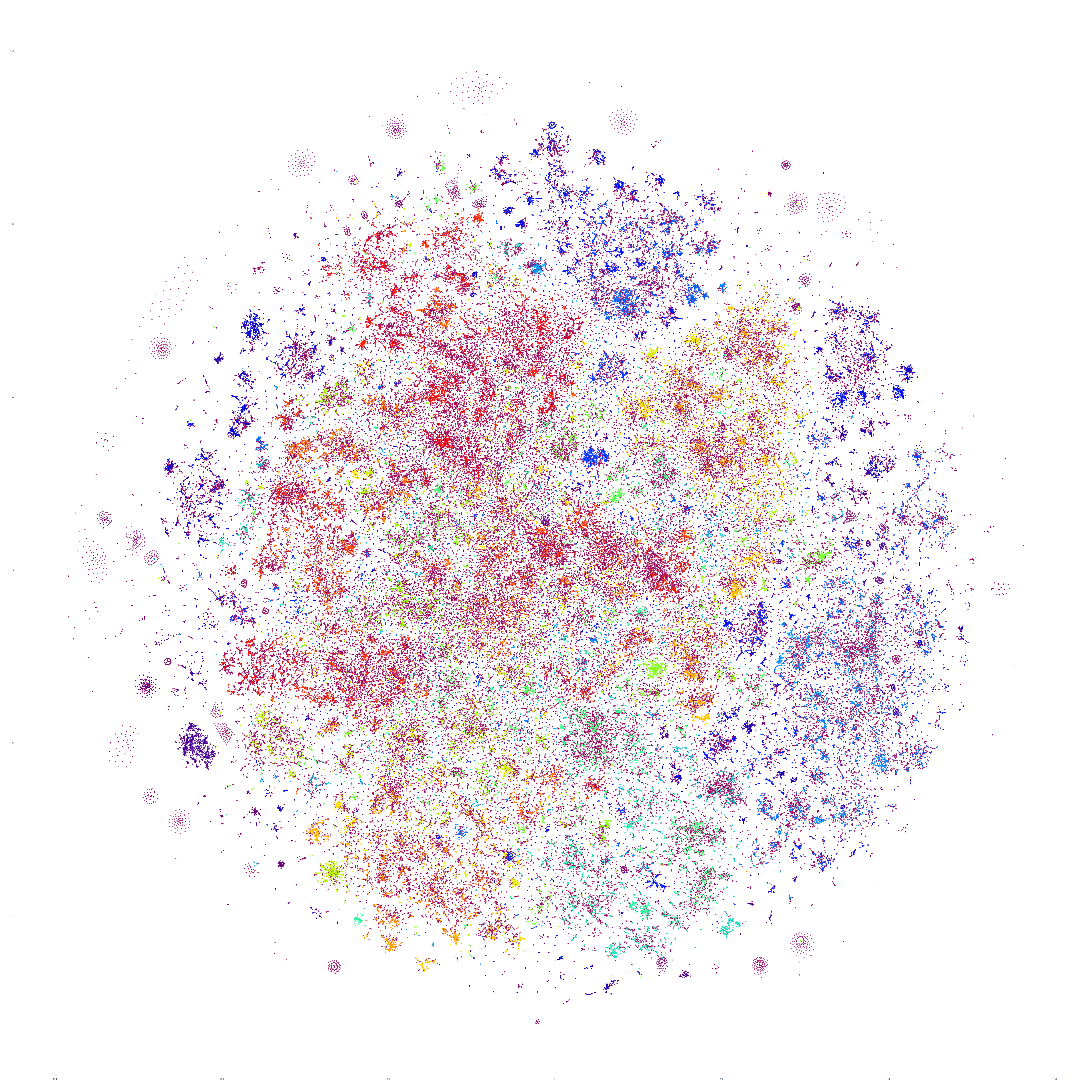
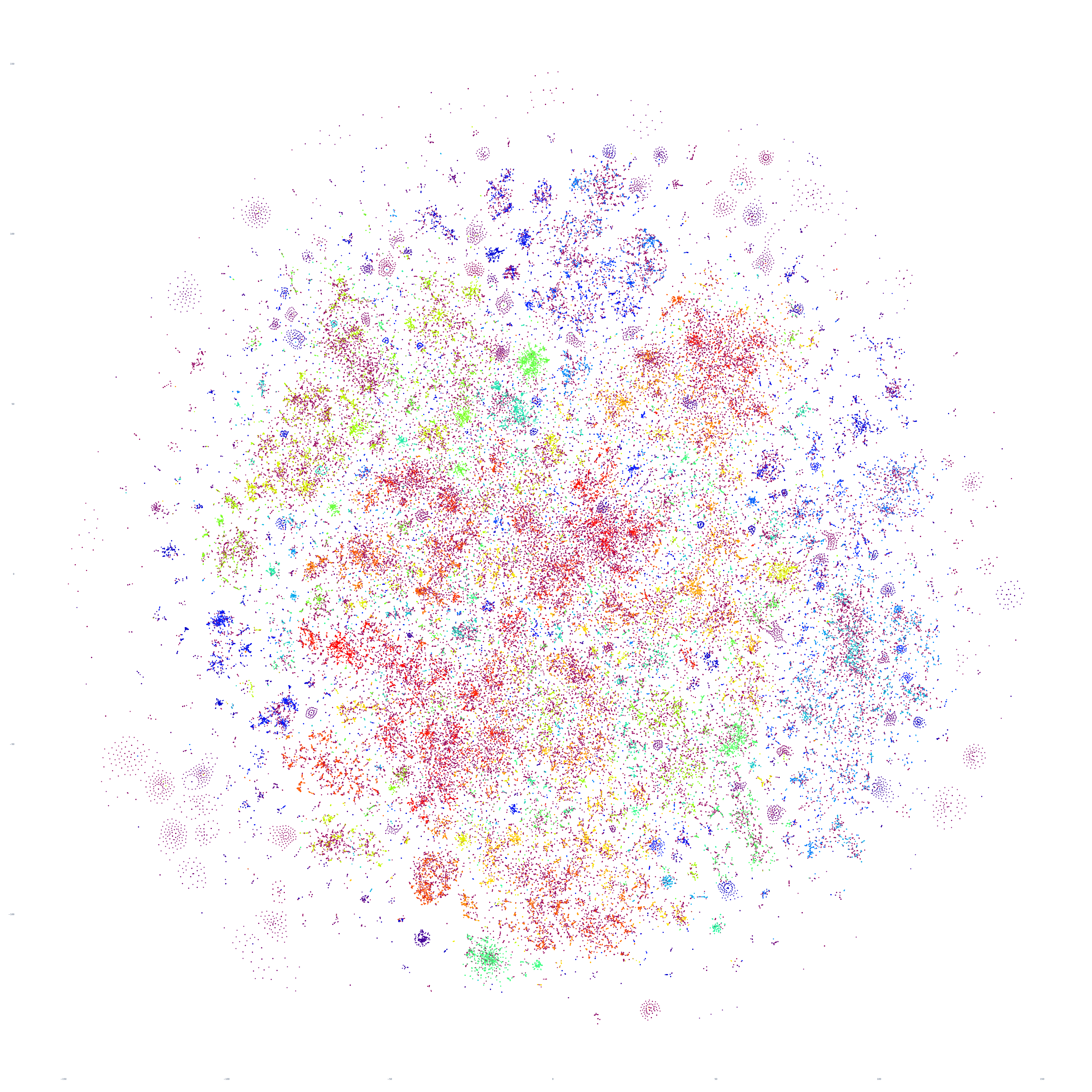
Rather than randomly coloring the article points, let's apply semantic clustering to our dataset, using HDBSCAN to group articles according to the similarity of their fulltext contents. Thus, our final graph will combine two layers: the color of points will groups them into related clusters of articles, while their positioning in the graph will separately capture the overall structural similarity amongst articles. Two layers of relatedness captured in a single graph.
Due to HDBSCAN's considerable computational requirements, we'll employ UMAP preprocessing to collapse the GSG's USEv4 512-dimension embeddings down to 10 dimensions to allow HDBSCAN to employ its optimized clustering path and to minimize as much as possible the total computation space.
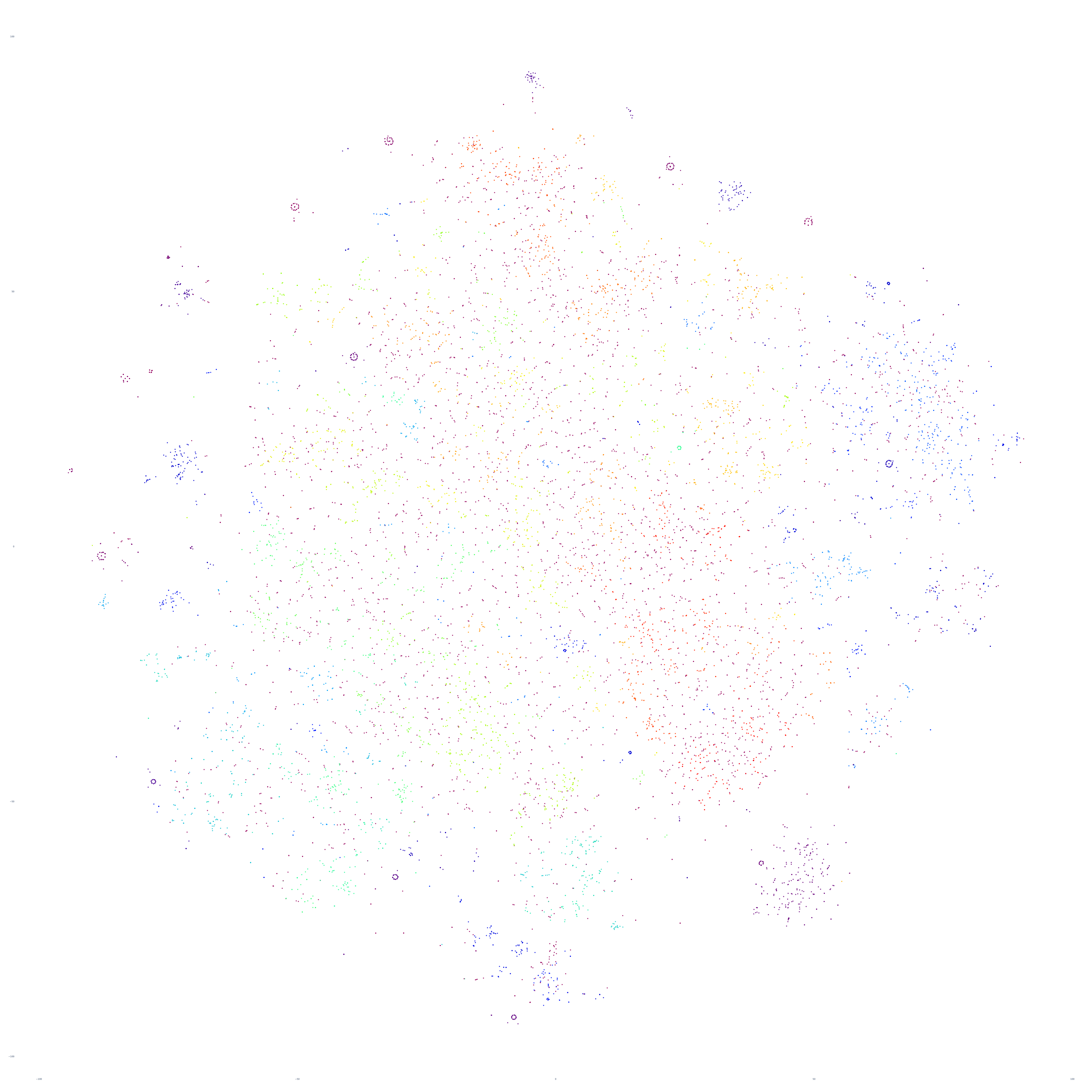
Let's start with a random sample of 500 articles. While the underlying computation occurs quickly, clearly this is too sparse to capture anything of meaning:

How about we increase the density to a random sample of 10,000 articles? Here we begin to see early glimmers of macro-level structure. Note that when HDBSCAN cannot find a sufficiently strong clustering for any given article, it marks it as "noise" and thus some of the diffuseness in the graph's coloration is from this "noise" category.
Let's increase that number to 100,000 articles. Here we begin to see the first glimmers of real structure emerge, with diffuse and intricate structures alike. Note how coloring, while tending to group together, is also somewhat diffuse. This typically represents either articles that belong to multiple groups having different associations under the two clustering algorithms or artifacts of the 2D projection used for visualization (or both). Note that we are using hard clustering here for coloration purposes, which forces each article into a single group, while HDBSCAN supports soft clustering (where articles can belong to multiple clusters – such as an article that discusses both the Israel-Hamas and Ukraine-Russia conflicts).
To make the underlying computation tractable, recall that we are using UMAP preprocessing to reduce the dimensionality down to 10 from 512. While pinning the layout in place, let's test using UMAP reduction to 25 dimensions, rather than 10, to see if the enhanced dimensionality improves clustering in any way. While the coloration of some points changes, the results are extremely minor.
Let's boost our density up to 200,000 articles. By doubling the number of articles considered, we see even more structure begin to appear:
How about increasing again to 300,000 articles? The structure doesn't change too much, but the internal clustering within the diffuse groupings becomes more apparent:
And finally, let's increase once more to 350,000 articles, which was the maximum we were able to render in this particular experiment due to an unknown failure state in the rasterization stage of our pipeline (Plotly's Kaleido rendering library), which will require further work to diagnose. Here we can see fascinating complex structure, with diffuse and tightly intricate clusters alike, representing a single day of the global news landscape.
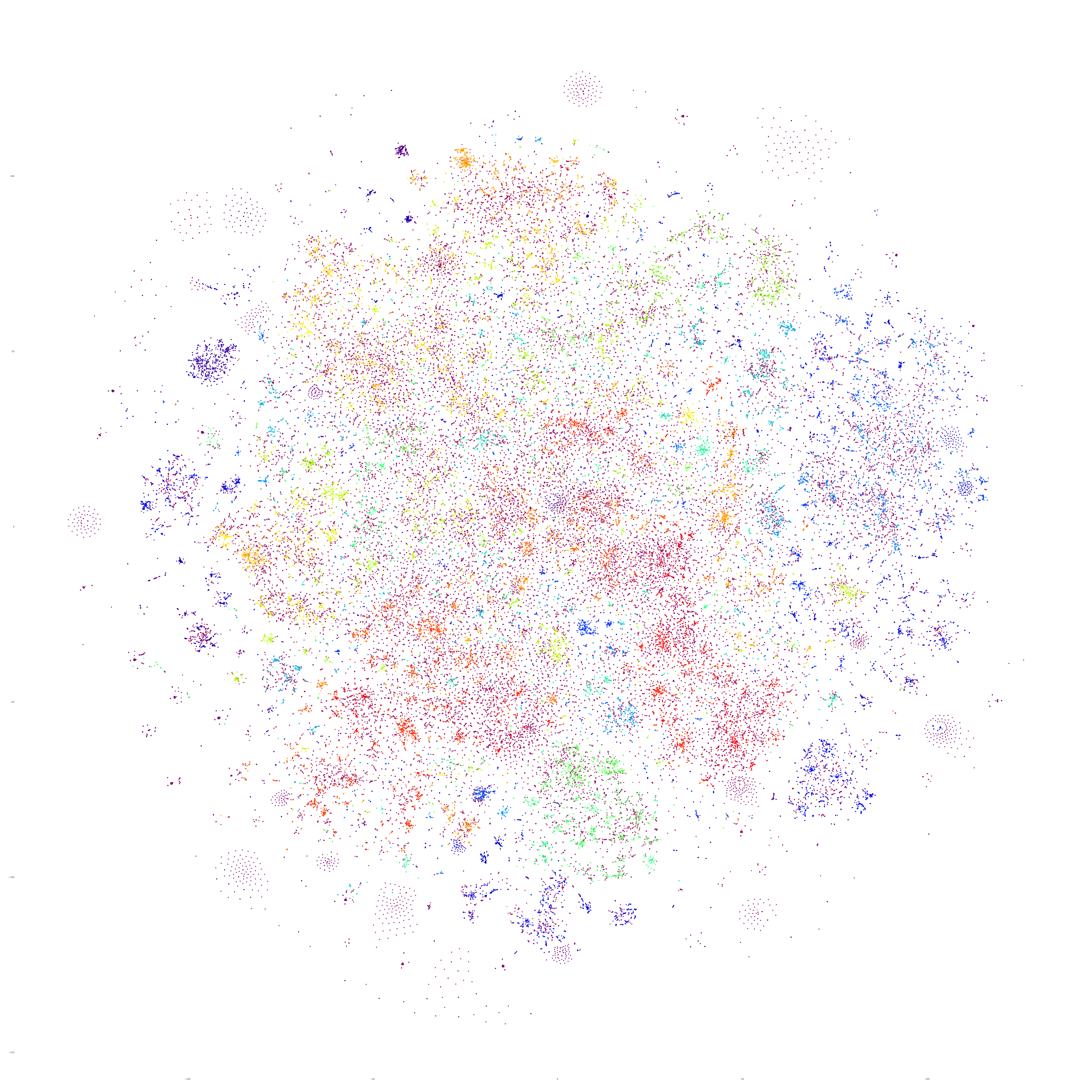
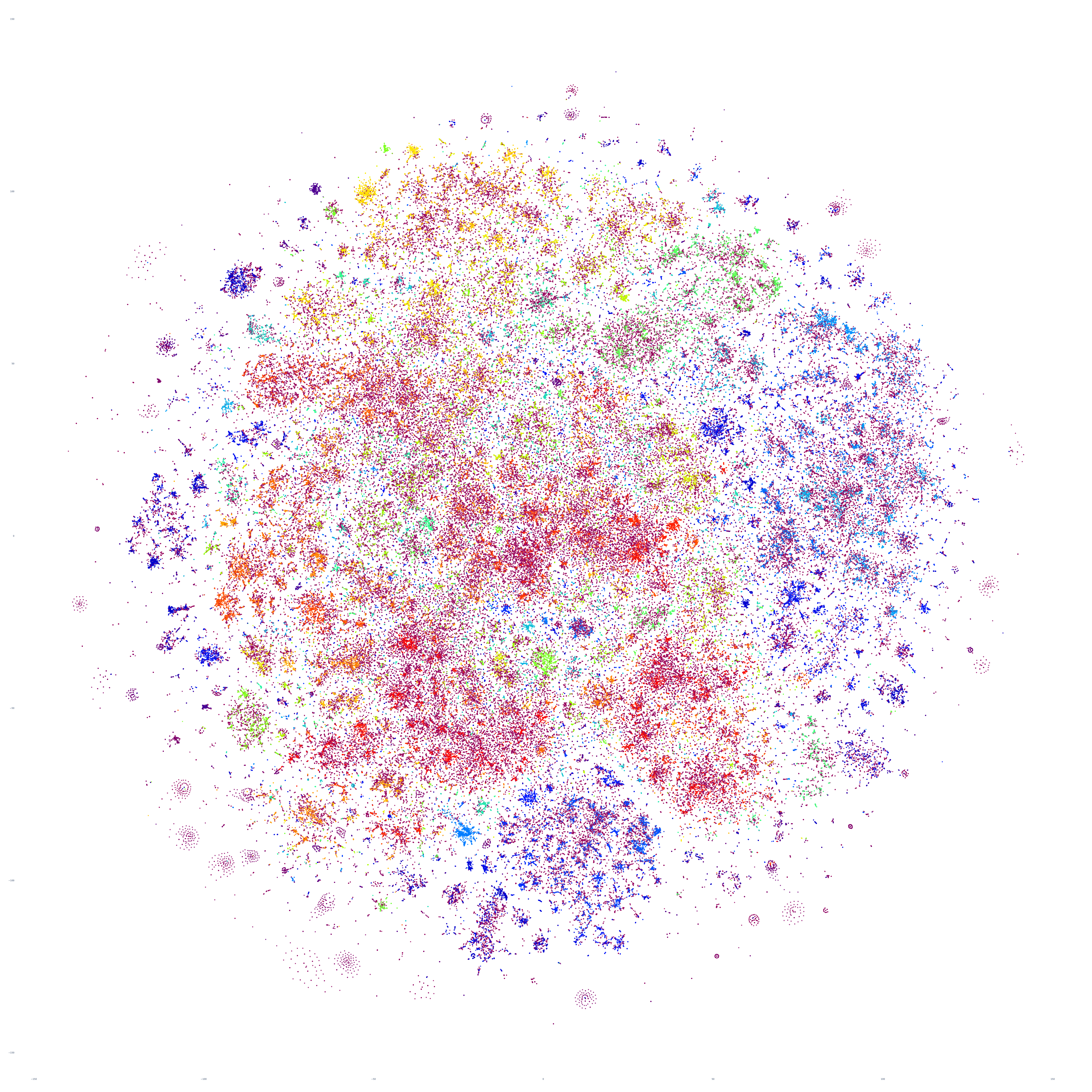
What if we repeat this process for the following day, October 18, 2023? Fascinatingly, the macro-level structure looks extremely similar, though with some very subtle variations:
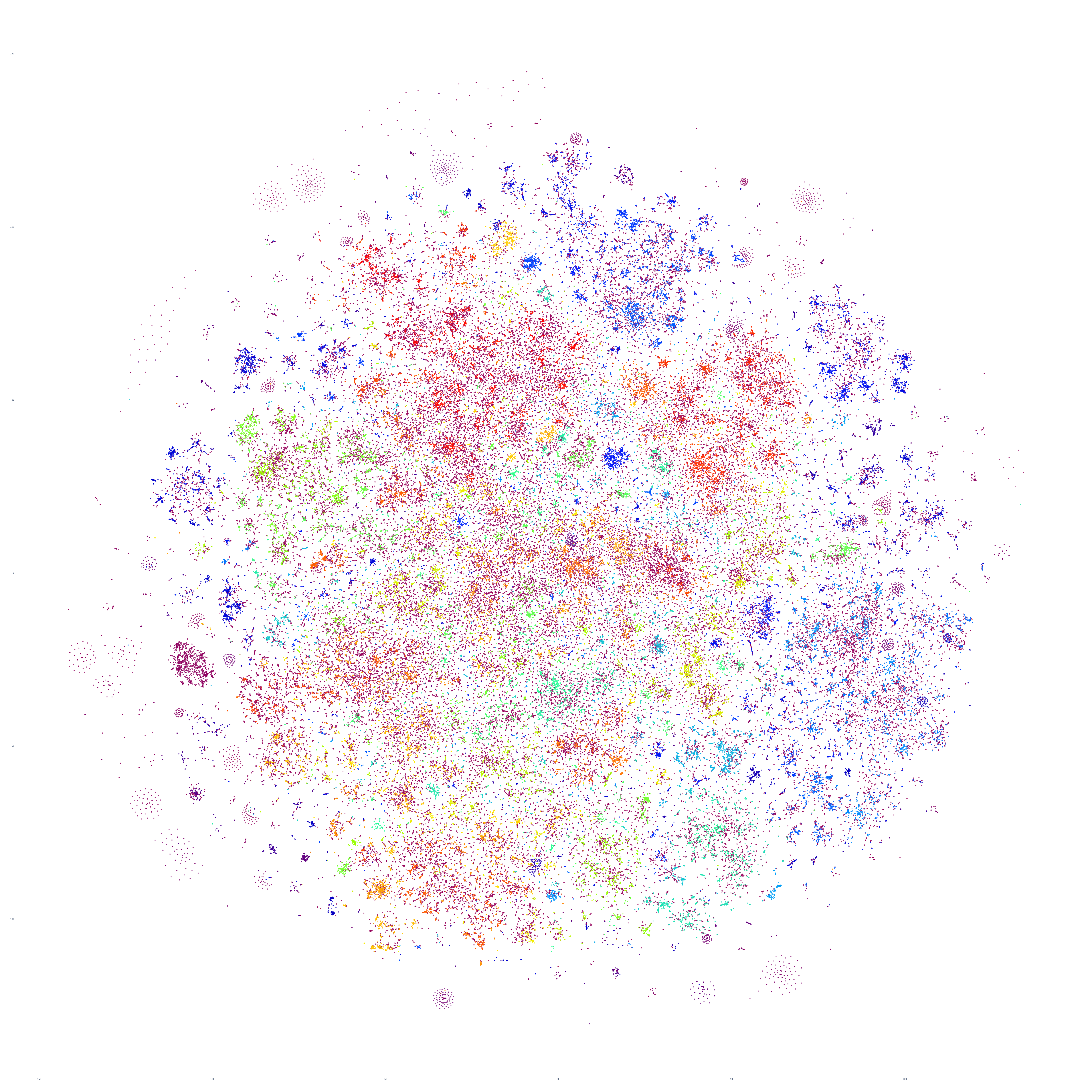
And October 19th? Once again, the results are extremely similar, with very small differences.
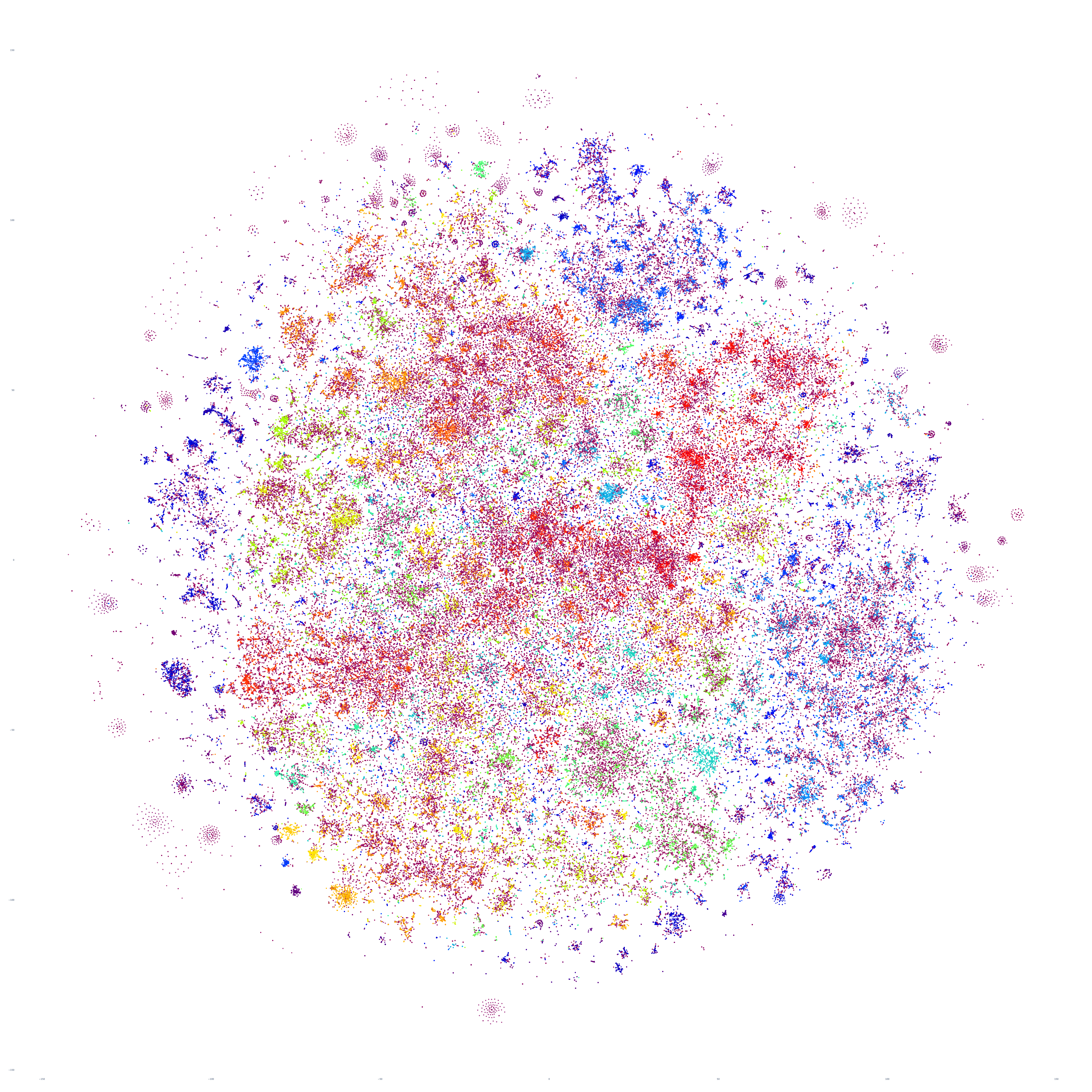
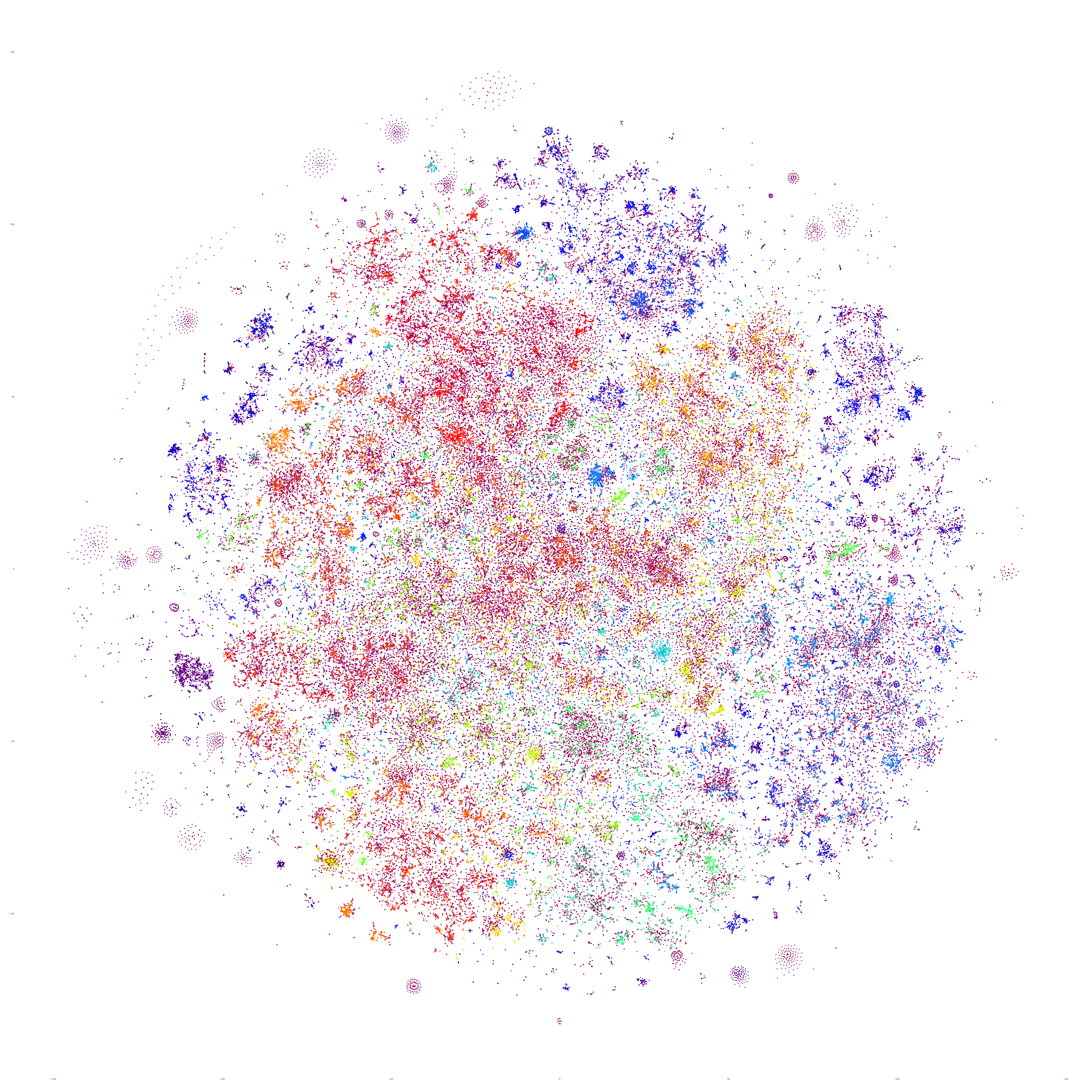
Perhaps the similarities are driven by the major news stories of that week, so let's repeat with September 20th – roughly one month prior. At first glance this graph appears extremely similar too, but there are a number of macro-level differences in its structure. This suggests that there is a certain level of uniformity to the daily news landscape in terms of macro-level structure, with the world's nations, cultures and citizenry forming a predictable tapestry of coverage, with the biggest international stories influencing that fabric sufficiently on a week-by-week basis to be visible in the greater uniformity of its structure.
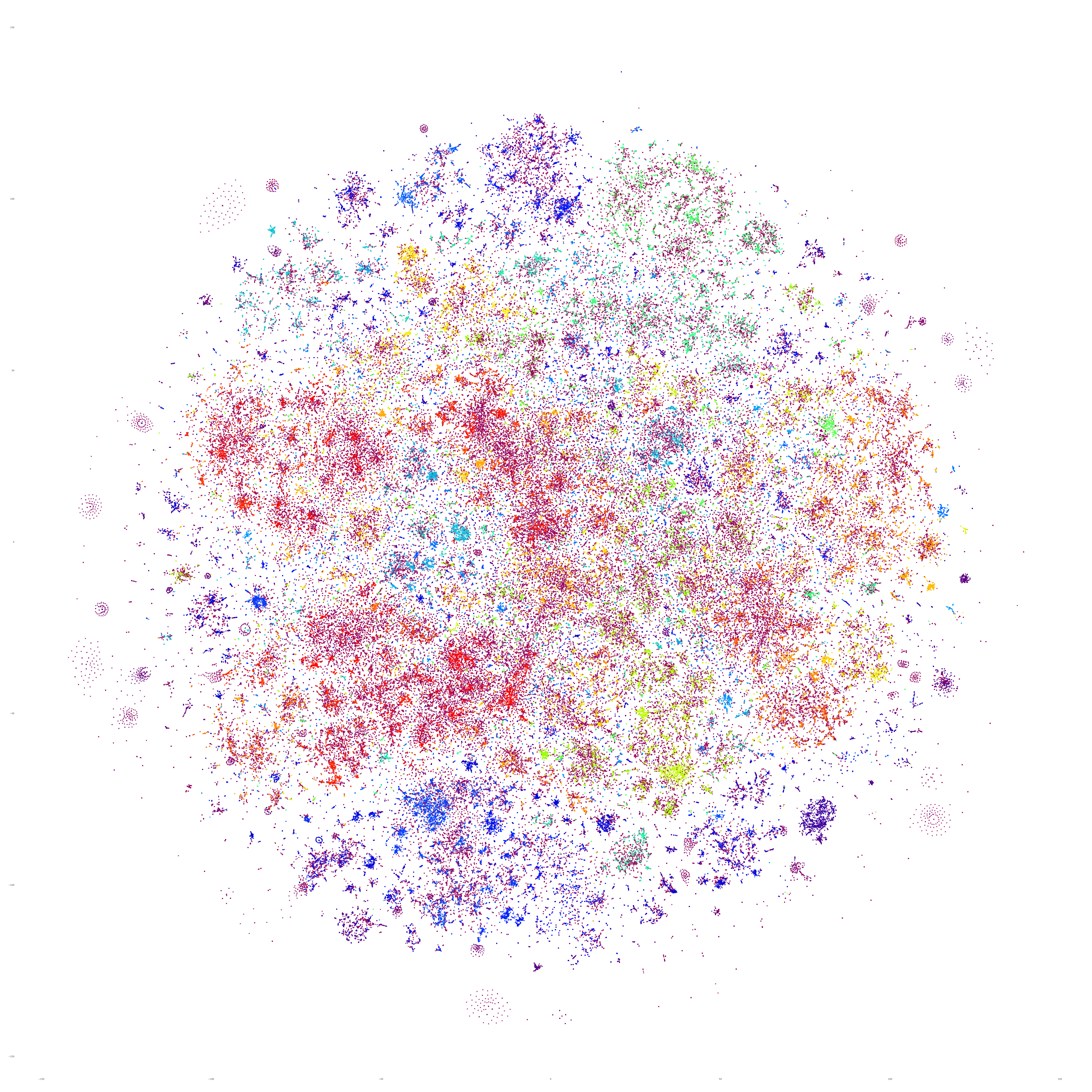
What if we return to October 17th and examine only its English-language coverage, excluding the 65 live-translated languages included in the earlier graphs? The resulting graph looks highly similar, though with greater micro-level clustering and differentiated stratification between clusters.
How did we generate these graphs?
First we'll download the GSG datasets for the given day:
#first we'll download all of the files from https://storage.googleapis.com/data.gdeltproject.org/gdeltv3/gsg_docembed/20231017*.gsg.docembed.json.gz TO ./CACHE/
#then unpack
time find ./CACHE/*.gz | parallel --eta 'pigz -d {}'
pigz -d ./CACHE/*
Then save the following Perl script to "collapse.pl". This script reads all of the individual minute-level GSG files and collapses them into a single daily-level file:
#!/usr/bin/perl

use JSON::XS;

open(OUT, ">./MASTER.json");
foreach $file (glob("./CACHE/*.json")) {
    open(FILE, $file);
    while() {
        my $ref; $ref = decode_json($_);
        if (!exists($SEEN{$ref->{'url'}})) {
            my $write; $write{'title'} = $ref->{'title'}; $write{'embed'} = $ref->{'docembed'}; $write{'lang'} = $ref->{'lang'};
            $write{'lang'}=~s/([\w']+)/\u\L$1/g;
            print OUT JSON::XS->new->allow_nonref(1)->utf8->encode(\%write) . "\n";
            $SEEN{$ref->{'url'}} = 1;
        }
    }
    close(FILE);
}
close(OUT);
Then we'll sample the data:
shuf -n 500 MASTER.json > MASTER.sample.json
shuf -n 10000 MASTER.json > MASTER.sample.json
shuf -n 100000 MASTER.json > MASTER.sample.json
shuf -n 200000 MASTER.json > MASTER.sample.json
shuf -n 350000 MASTER.json > MASTER.sample.json

#for our English-only sample:
grep '"English"' MASTER.json > MASTER.json.english
shuf -n 350000 MASTER.json.english > MASTER.sample.json
Install some needed libraries:
pip install umap-learn
And save the following Python script as "run.py". You'll notice that to make the HDBSCAN computation more tractable, we use UMAP dimensionality reduction. This tends to yield results than PCA reduction.
#########################
#LOAD THE EMBEDDINGS...

import numpy as np
import matplotlib.pyplot as plt
from PIL import Image
import jsonlines
import multiprocessing

# Load the JSON file containing embedding vectors
def load_json_embeddings(filename):
    embeddings = []
    titles = []
    langs = []
    with jsonlines.open(filename) as reader:
        for line in reader:
            embeddings.append(line["embed"])
            titles.append(line["title"])
            langs.append(line["lang"])
    return np.array(embeddings), titles, langs

json_file = "MASTER.sample.json"
embeddings, titles, langs = load_json_embeddings(json_file)
len(embeddings)

import hdbscan
import umap
import time
def cluster_embeddings(embeddings, min_cluster_size=5):
    start_time = time.process_time()
    embeddings_reduced = umap.UMAP(n_neighbors=30,min_dist=0.0,n_components=10,verbose=True).fit_transform(embeddings)
    end_time = time.process_time()
    elapsed_time = end_time - start_time
    print(f"UMAP: : {elapsed_time} seconds")
    start_time = time.process_time()
    clusterer = hdbscan.HDBSCAN(min_cluster_size=min_cluster_size, core_dist_n_jobs = multiprocessing.cpu_count())
    clusters = clusterer.fit_predict(embeddings_reduced)
    end_time = time.process_time()
    elapsed_time = end_time - start_time
    print(f"HDBSCAN: : {elapsed_time} seconds")
    return clusters

clusters = cluster_embeddings(embeddings, 5)
#########################
#VISUALIZE...

from sklearn.manifold import TSNE
from sklearn.decomposition import PCA
import plotly.graph_objs as graph
import plotly.io as pio

def plotPointCloud(embeddings, clusters, titles, langs, title, algorithm):
    if (algorithm == 'PCA'):
        pca = PCA(n_components=2, random_state=42)
        embeds = pca.fit_transform(embeddings)
    if (algorithm == 'TSNE'):
        tsne = TSNE(n_components=2, random_state=42)
        embeds = tsne.fit_transform(embeddings)

    unique_clusters = np.unique(clusters)
    print("Clusters: " + str(unique_clusters))

    trace = graph.Scatter(
        x=embeds[:, 0],
        y=embeds[:, 1],
        marker=dict(
            size=6,
            #color=np.arange(len(embeds)), #color randomly
            color=clusters, #color via HDBSCAN clusters
            colorscale='Rainbow',
            opacity=0.8
        ),
        #text = langs,
        #text = titles,
        #text = [title[:20] for title in titles],
        hoverinfo='text',
        #mode='markers+text',
        mode='markers',
        textposition='bottom right'
    )

    layout = graph.Layout(
        #title=title,
        xaxis=dict(title=''),
        yaxis=dict(title=''),
        height=6000,
        width=6000,
        plot_bgcolor='rgba(255,255,255,255)',
        hovermode='closest',
        hoverlabel=dict(bgcolor="black", font_size=14)
    )

    fig = graph.Figure(data=[trace], layout=layout)
    fig.update_layout(autosize=True)

    # Save the figure as a PNG image
    pio.write_image(fig, 'output.png', format='png')

# Call the function with your data
#clusters = []
plotPointCloud(embeddings, clusters, titles, langs, 'Title', 'TSNE')
#########################
Then run the following command with each variation of "MASTER.sample.json" to visualize it:
time python3 ./run.py
In terms of runtime on a 64-core N1 GCE VM with 400GB RAM:
- 500 articles: 0m18s
- 10K articles: 1m29s
- 100K articles: 7m29s
- 200K articels: 20m24s
- 300K articles: 29m26s
- 350K articles: 38m46s
This represents just an initial experiment with at-scale analysis of an entire day of global news coverage – stay tuned for more in this series.