Yesterday we explored how, in an ever more unstable world, we can use multimodal image embedding models to cluster, search, visualize, gain new insights and better understand the underlying visual storytelling narratives of domestic television news around the world – in this case the parallel universe of Russian narratives about its invasion of Ukraine. How might we scale yesterday's experiment with a single 30-minute segment up to an entire day of airtime, visualizing at scale a complete 24 hours of Russia's domestic narratives and the visual metaphors it is using to portray the invasion and global events to the Russian population?
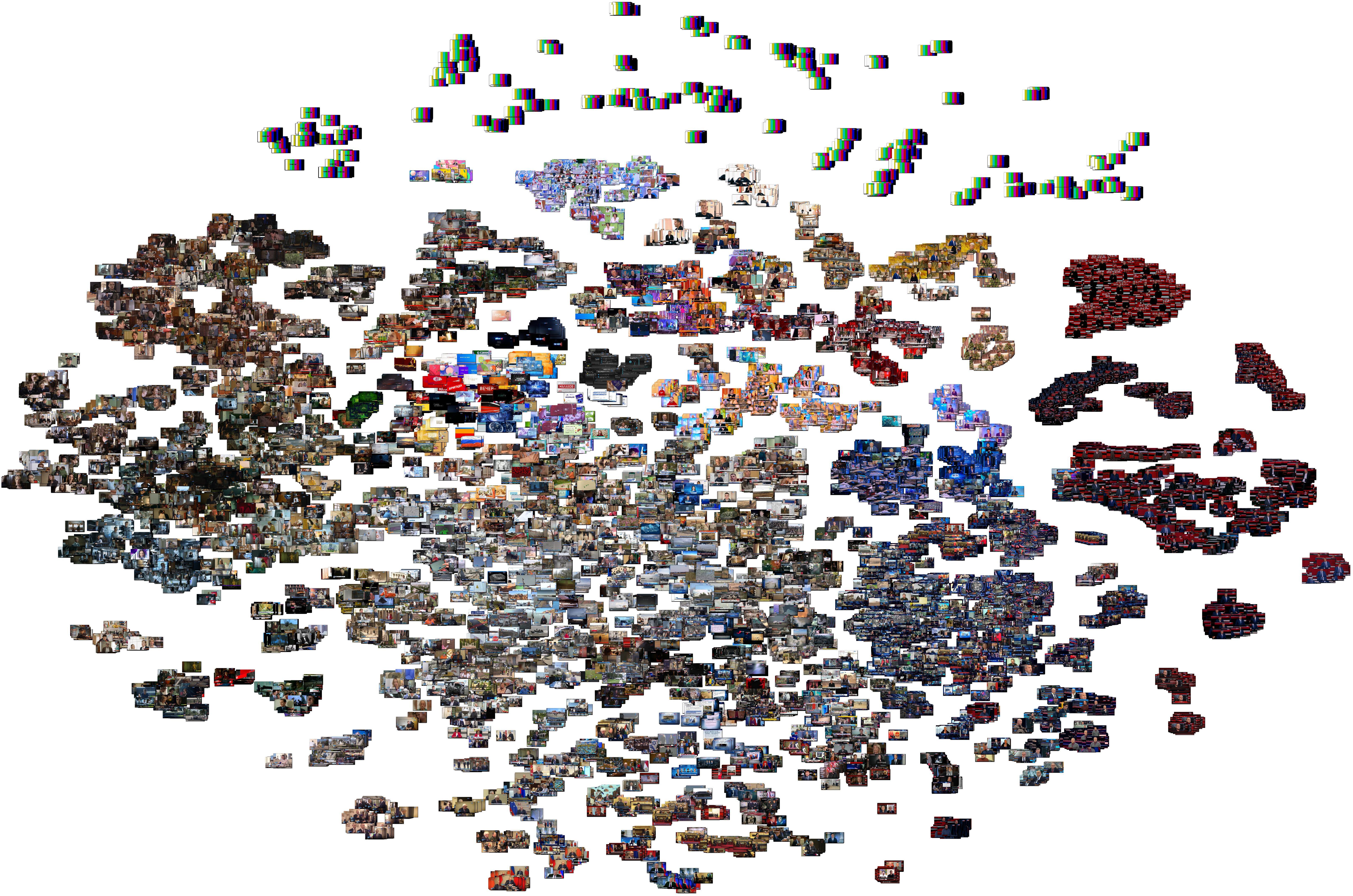
One of the most powerful elements of yesterday's analysis were the two visualizations that examined the broadcast as a clustered image cloud, grouping it into distinct thematic groupings via PCA and t-SNE, offering an at-a-glance look at the visual narrative landscape of the broadcast. What does it look like to scale that up to an entire day?
The end results suggest there is intriguing promise in this kind of landscape visualization, not least in the ability to identify tight thematic clusters, isolated narratives and the kinds of color schemes and representations used. Unsurprisingly, PCA offers the best global-scale understanding of color and thematic distribution, but yields a clustering that makes it difficult to extract higher-order meaning beyond those basics. t-SNE clustering offers the most actionable insights, more readily distinguishing through spatial distribution the visual narrative focus of the day and especially the relatedness of "similar but different enough" clusters. Interestingly, there are definite color schema distributions representing different kinds of topics that are highly distinguishable in these visualizations, suggesting color histograms might be a useful heuristic for distinguishing certain kinds of topics as a prefiltering optimization for certain kinds of image assessment tasks. One powerful enhancement would likely be to overlay image captioning and other textual-descriptive insights onto the visualization and use them for additional topically discriminative segmentation and separation tasks to make some of the denser clusters more stratified and lend additional insight into the meaning behind others.
As with yesterday's experiment, we'll use GCP's Vertex AI Multimodal Embedding model. Since the model automatically resizes images down to 512×512, we'll go ahead and do that ourselves to save on bandwidth and latency. In a production application, this could also offer the opportunity to customize the resizing pipeline to a tailored application-specific workflow that optimizes or enhances specific details to focus the model's attention on, etc. Alternatively, it might be better to leave the resizing to the API, since one might assume it uses a resizing workflow custom-built to yield optimal results – you should experiment based on your own latency, bandwidth and other needs.
#resize all of the images...
time find ./IMAGES/ -depth -type f -name '*.jpg' | parallel --eta 'convert {} -resize 512x512\> {.}.resized.jpg'

#compute all of the embeddings... (edit script to change to your GCP Project ID)
wget https://storage.googleapis.com/data.gdeltproject.org/blog/2023-multimodalembeddingexperiments/exp_makeimageembed_vertex.pl
chmod 755 *.pl
time find ./IMAGES/ -depth -type f -name '*.resized.jpg' | parallel --eta -j 2 './exp_makeimageembed_vertex.pl {}'

#merge the embeddings into a single file per broadcast...
wget https://storage.googleapis.com/data.gdeltproject.org/blog/2023-multimodalembeddingexperiments/exp_makeimageembed_vertex_mergeembeddings.pl
chmod 755 *.pl
time find ./IMAGES/ -mindepth 1 -type d | parallel --eta './exp_makeimageembed_vertex_mergeembeddings.pl {}'

#combine into a single JSON file for the entire day...
cat IMAGES/*.json > RUSSIA1_20231017-FULLDAY.embeds.json
You can skip all of that and download our pre-computed full-day embedding file:
Now let's visualize the complete day through PCA, t-SNE and PCA-assisted t-SNE. Save the following script to "visualize.py" and run via "python3 ./visualize.py". Note that this requires 40GB of RAM and due to Python memory management and garbage collection, you may need to run three times, each time with just one of the plotImageCloud() calls at the bottom of the script, instead of calling all three in sequence in a single script, to avoid exhausting available memory resources.
#########################
#LOAD THE EMBEDDINGS...

import numpy as np
import matplotlib.pyplot as plt
from PIL import Image
import jsonlines
import hdbscan

# Load the JSON file containing embedding vectors
def load_json_embeddings(filename):
    embeddings = []
    image_filenames = []
    with jsonlines.open(filename) as reader:
        for line in reader:
            embeddings.append(line["embed"])
            image_filenames.append(line["imagefilename"])
    return np.array(embeddings), image_filenames

json_file = "RUSSIA1_20231017-FULLDAY.embeds.json"
embeddings, image_filenames = load_json_embeddings(json_file)
#########################
#VISUALIZE THE EMBEDDINGS...

from sklearn.manifold import TSNE
from sklearn.decomposition import PCA
import matplotlib.pyplot as plt

def plotImageCloud(embeddings, image_filenames, title, algorithm, outfilename):
    if (algorithm == 'PCA'):
        pca = PCA(n_components=2, random_state=42)
        embeds = pca.fit_transform(embeddings)
    if (algorithm == 'TSNE'):
        tsne = TSNE(n_components=2, random_state=42)
        embeds = tsne.fit_transform(embeddings)
    if (algorithm == 'PCATSNE'):
        embeds = PCA(n_components=50, random_state=42).fit_transform(embeddings)
        embeds = TSNE(n_components=2, random_state=42).fit_transform(embeds)

    f = plt.figure(figsize=(90, 60))
    ax = plt.subplot(aspect='equal')
    sc = ax.scatter(embeds[:,0], embeds[:,1])
    _ = ax.axis('off')
    _ = ax.axis('tight')

    from matplotlib.offsetbox import OffsetImage, AnnotationBbox
    for i in range(len(image_filenames)):
        image = Image.open(image_filenames[i])
        im = OffsetImage(image, zoom=0.10)
        ab = AnnotationBbox(im, embeds[i], xycoords='data', pad=0.00)
        ax.add_artist(ab)

    #plt.title(title) #remove title to maximize pixel space...
    #plt.show()
    plt.savefig(outfilename)


#compare PCA and TSNE... NOTE: this requires 40GB+ RAM and may require running one at a time due to Python memory management
plotImageCloud(embeddings, image_filenames, 'PCA Clustering', 'PCA', './pca.jpg')
#plotImageCloud(embeddings, image_filenames, 'TSNE Clustering', 'TSNE', './tsne.jpg')
#plotImageCloud(embeddings, image_filenames, 'PCA-TSNE Clustering', 'PCATSNE', './pcatsne.jpg')
#########################
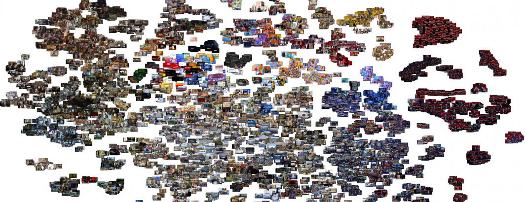
After generating the graphs, ImageMagick is used to trim the surrounding whitespace in the margins, since there is typically several inches of blank space on all sides framing the plot:
convert pca.jpg -trim pca-trim.jpg
convert tsne.jpg -trim tsne-trim.jpg
convert pcatsne.jpg -trim pcatsne-trim.jpg
In terms of speed, PCA should be the fastest, while t-SNE is known to be more computationally expensive. PCA-assisted t-SNE is an approach recommended by some organizations as a way to accelerate t-SNE for high-dimension embeddings like Vertex's multimodal embeddings by first collapsing the dimensionality from 1,408 down to 50, greatly reducing the clustering space for t-SNE. We manually set "random_state" for all three algorithms so that the seed conditions are always the same, ensuring the results are stable across runs for debugging and tuning purposes – in a production application you might change this to be able to yield different results. Here we ran on a 64-core VM, but only t-SNE was able to use more than a single core and only utilized 4 of the cores for a short period.
The final runtimes, averaged across 5 runs each can be seen below. In this case, PCA-assisted t-SNE yields only an imperceptible speed increase and as seen in a moment, highly similar results. In larger applications it may yield more existentially important speedups, but here the majority of time was spent in the rendering and image construction stage. One downside of using PCA preclustering with t-SNE is that it results in smaller clusters that lose some of their interconnectedness, but that could be a benefit in some applications and likely could be adjusted by experimenting with the requested dimensionality reduction of the PCA preprocessing stage.
- PCA: 4m49s
- t-SNE: 5m27s
- PCA-Assisted t-SNE: 5m20s
PCA Clustering
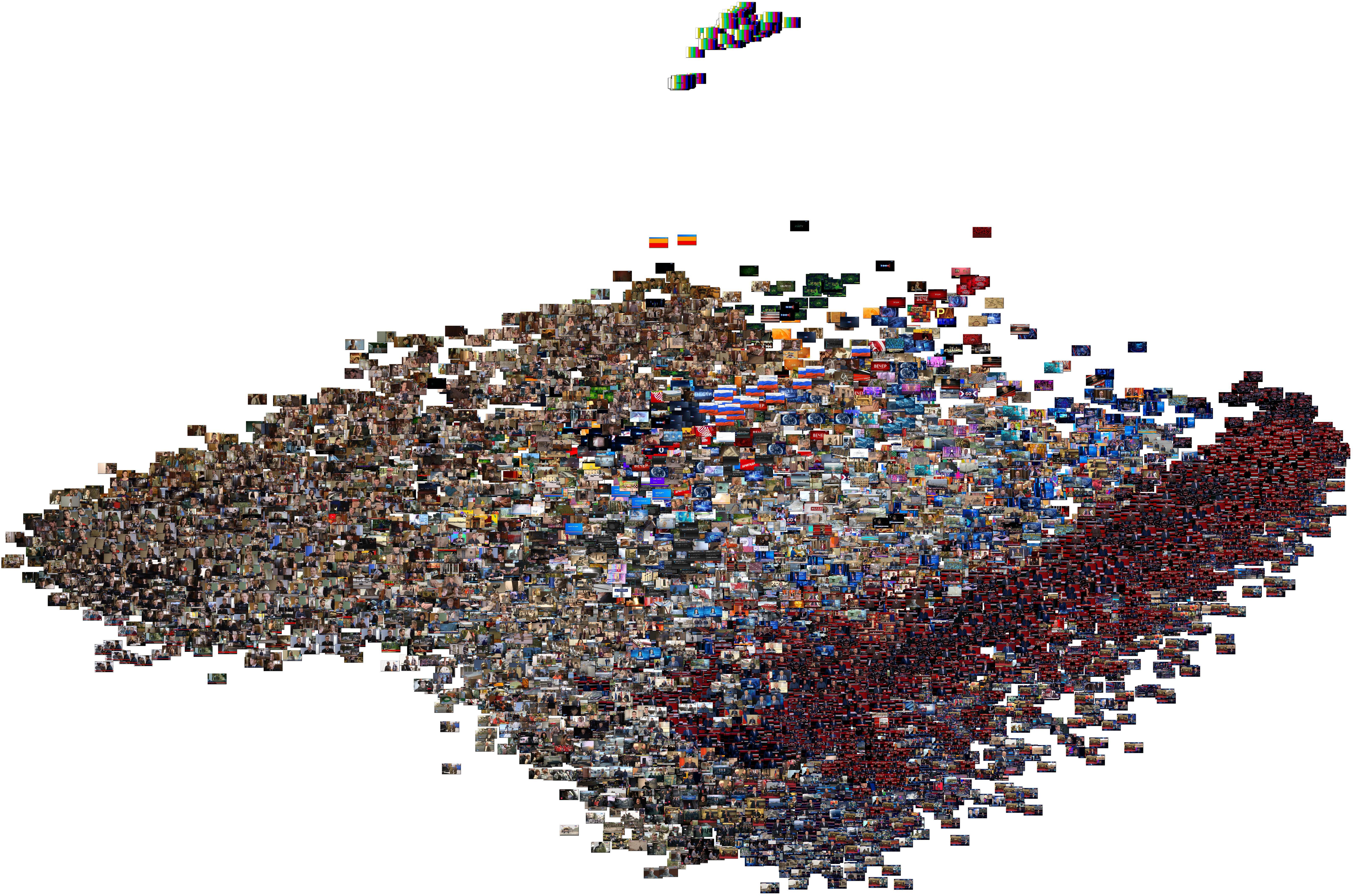
t-SNE Clustering
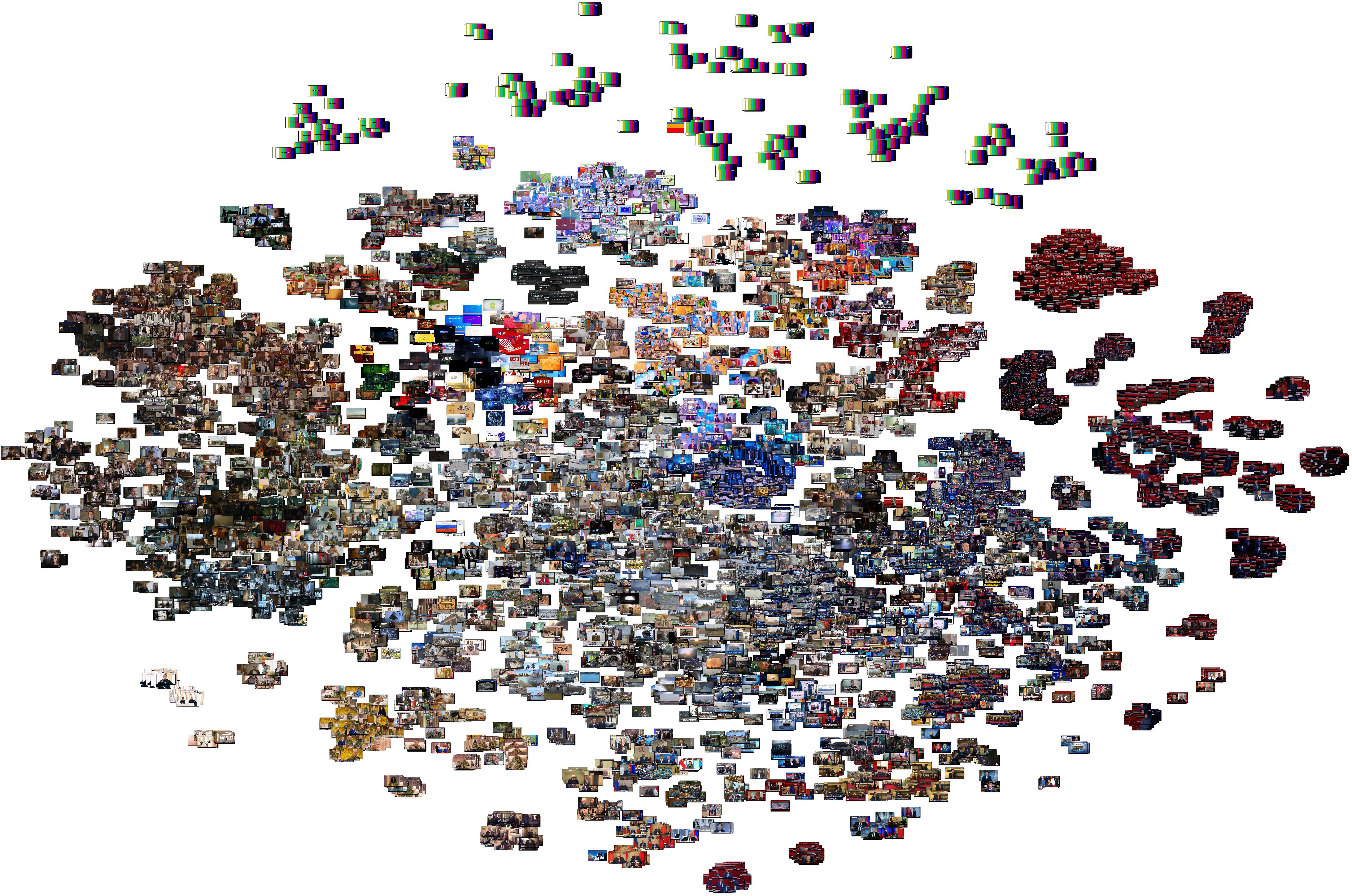
PCA-Assisted t-SNE Clustering