Earlier this year we used Google's Cloud Video, Cloud Vision, Cloud Speech to Text and Cloud Natural Language APIs to "watch" a week of television news from CNN, MSNBC and Fox News, along with the morning and evening broadcasts of ABC, CBS, NBC and PBS from the Internet Archive's Television News Archive to explore how AI sees television news and what new insights such analyses could yield.
One of the analyses we explored involved sampling the 2,916,729 seconds of airtime into one frame per second still images, which were then analyzed through the Cloud Vision API, allowing us to crowdsource the open web's captioning of similar images to connect the online and television worlds.
This analysis yielded a dataset of 27,854,949 total Web Entity annotations which co-occurred 143,834,082 times in 6,099,191 distinct pairings.
What might it look like to visualize this co-occurrence network and how might it help us to better understand a week of television news?
Following in the footsteps of the enormous 3.8-billion-edge Web Entity co-occurrence graph we created last week from half a billion online images spanning three years, using the same approach, a single SQL query and just 57 seconds was all that was required to process the "Web Entities" summary file for the week of television news into a co-occurrence graph in Gephi's edge list format.
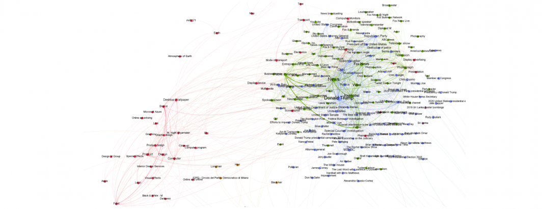
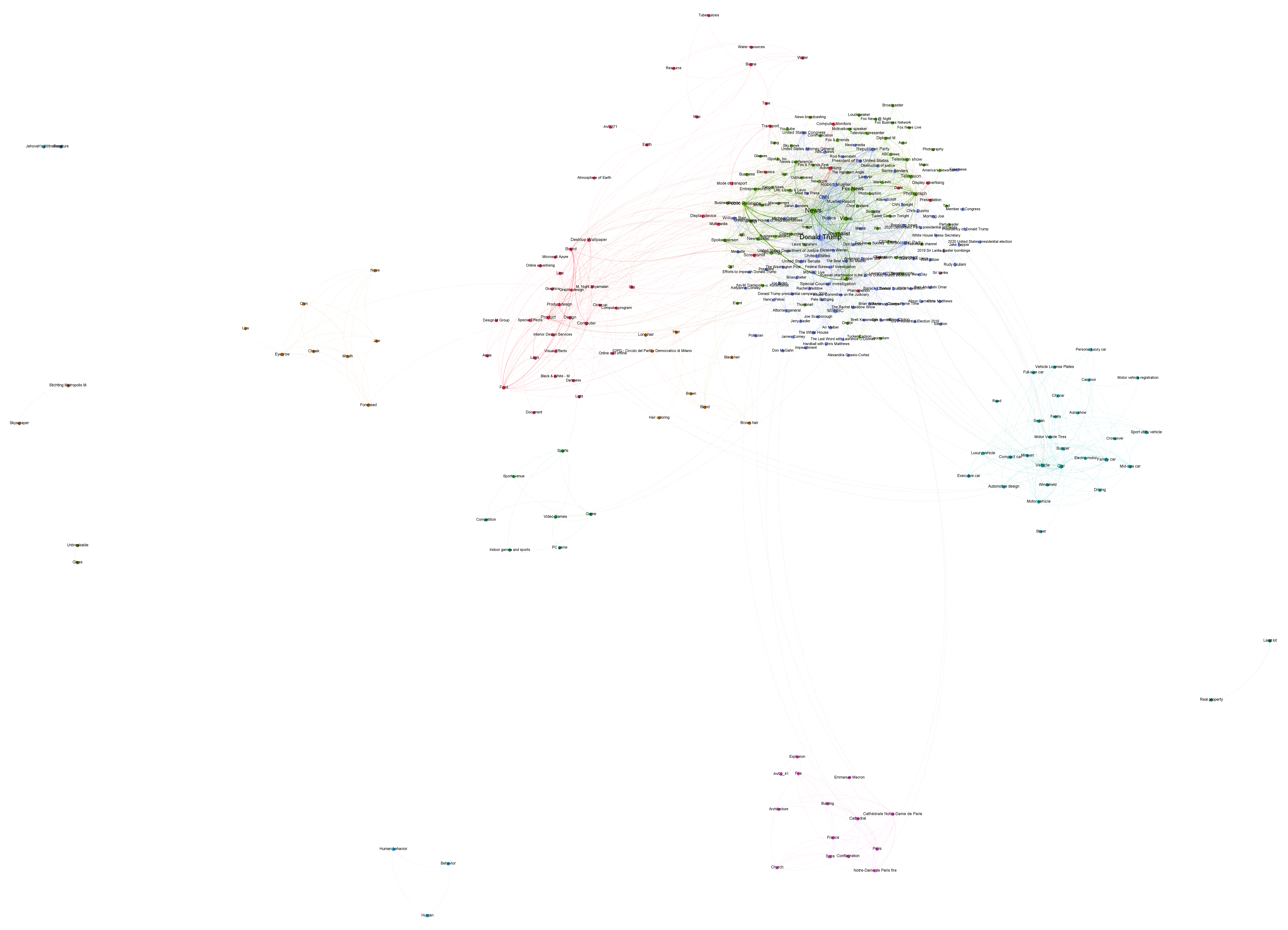
The visualization below shows the 1,500 strongest co-occurrences in that graph. The week chosen, April 15 to April 22, 2019, contained two major stories: the Mueller investigation and the Notre Dame Cathedral fire.
Look closely at the graph below and you will see the core cluster at top right contains Donald Trump, the Mueller investigation and an array of other politics and related news events from that week.
Beneath it at the bottom of the graph is the cluster of topics covering the Notre Dame Cathedral fire. Its self-contained isolated cluster reflects the fact that it was a high-intensity self-contained story that did not relate to other stories being covered during that week.
To the right and below the main cluster is a vehicle-related cluster reflecting car commercials, while the red cluster to the bottom left of the core reflects common scene transition and textual overlays used in commercials, while to its left is a cluster of human face components reflecting the human face zooming popular on television, while below it are sports-related commercials.
The fact that commercial-related topical clusters are so clearly isolated from the core and fall into such well-defined clusters suggests such semantic insights could be used to verify commercial identification algorithms, while the isolated nature of the Notre Dame Cathedral story offers insights into how "central" versus "isolated" stories could be identified.
The visualization files for this "top 1,500" graph can be downloaded below:
- Full Resolution 4K x 4k Graph With Labels.
- Full Resolution PDF Graph With Labels.
- Gephi File.
- CSV Edge List.
The master graph of all 6 million edges can be downloaded below:
We're tremendously excited to see what you're able to do with this powerful new graph representation!
TECHNICAL DETAILS
To create the graphs above, we used the "Web Entities" summary file from the "Vision AI Summaries" datasets. This is a gzipped tar file containing a list of files, one per broadcast that contains one row per 1fps image frame, with the first column being the frame number and the second column containing a semicolon-delimited list of the Web Entities found by the Cloud Vision API in that frame.
We simply cat'd all of those files into a single master file and loaded it into a temporary BigQuery table. Since the frameid column is local to each file, we first needed to make a new version of the table with globally unique IDs for each frame. Thankfully, BigQuery has a "GENERATE_UUID()" function that does precisely this, allowing us to simply run a "select all" from the first table and create a second table with the frameid replaced with a globally unique ID:
SELECT GENERATE_UUID() UUID, webentities FROM `TEMPTABLE1`
Then it was simply a matter of using our standard network construction code, courtesy of the ever-incredible Felipe Hoffa, to construct the final co-occurrence graph.
SELECT Source, Target, Count FROM (
SELECT a.entity Source, b.entity Target, COUNT(*) as Count
FROM (

(select UUID, entity from (
WITH nested AS (
SELECT UUID, SPLIT(webentities,';') entities FROM `TEMPTABLE2`
) select UUID, entity from nested, unnest(entities) entity
))

) a
JOIN (

(select UUID, entity from (
WITH nested AS (
SELECT UUID, SPLIT(webentities,';') entities FROM `TEMPTABLE2`
) select UUID, entity from nested, unnest(entities) entity
))

) b
ON a.UUID=b.UUID
WHERE a.entity<b.entity
GROUP BY 1,2
)
That's it! The output of the query above is a Gephi edge list, ready to subset and import directly into Gephi for visualization!