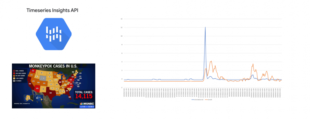
From capturing the first flickers of 2014's Ebola outbreak to powering one of the earliest alerts of the Covid-19 pandemic, GDELT's vast global realtime streams span every corner of the globe in 150 languages and climbing, capturing the earliest glimmers of disease outbreaks across the world where they are least expected. Last June we explored how Google's Timeseries Insights API could be applied to GDELT's Global Entity Graph, TV NGrams and Global Knowledge Graph to flag the earliest glimmers of tomorrow's biggest stories, but the approaches it presented were limited by the constraints of those datasets. With the release of the Web NGrams 3.0 dataset this past December, we now have the ability to perform generalized anomaly detection at planetary scale.
Today we'll showcase just how easy it is to create a realtime planetary-scale anomaly detection system for disease early warning and horizon scanning that combines the Timeseries Insights API, Web NGrams 3.0, Translation AI API and BigQuery into a single pipeline that flags the early stages of the coming global monkeypox outbreak this past May.
Monkeypox Early Warning
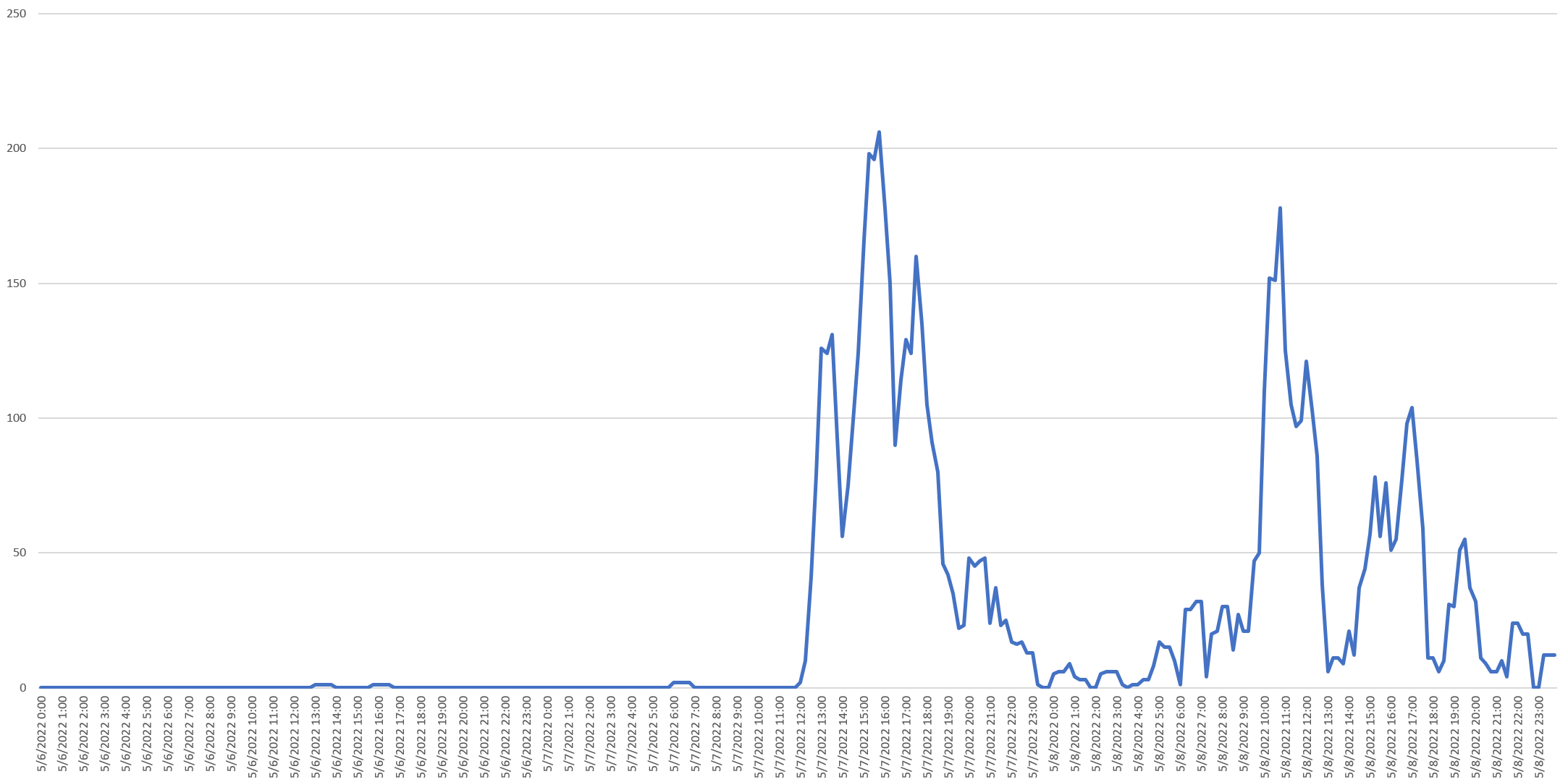
The May 2022 monkeypox outbreak represents a straightforward example of anomaly detection. Despite being endemic in parts of the world, monkeypox receives little media attention globally. When the initial known UK case was confirmed to the WHO on May 7, 2022, a vertical burst of media attention followed beginning at noon UTC, as can be seen in the following timeline of mentions from May 6 to May 8, 2022:
How might we create a fully automated system that can monitor GDELT's global monitoring streams from around the world in realtime for a catalog of infectious diseases and detect an emerging outbreak like this completely autonomously?
Creating The List Of Monitoring Terms
First, we'll need a list of keywords and keyphrases that represent the topic we want to monitor. For our demonstration pipeline here, we will provide the monitoring terms in English and then translate them into all of the languages GDELT monitors.
Start by creating a file called "WORDLIST.TXT" that contains the list of words and phrases that capture the topic we are interested in – in this case monkeypox. Since this will be used to perform an exact match, we need to capture all of the forms the word might appear in, including all conjugations if it is a verb, etc. In this case, a quick manual review of monkeypox coverage from previous years suggests it appears in both one word ("monkeypox") and two word ("monkey pox") forms so we will include both:
monkeypox
monkey pox
You can download the file:
Translating The Terms
The Web NGrams 3.0 dataset currently spans 150 languages. Most GDELT datasets like the GKG rely on GDELT's Translingual infrastructure to machine translate coverage from other languages into English for processing. Translation, whether done by machine or human, can alter the meaning or connotations of text, especially across highly dissimilar languages. From idiomatic expressions to words without a direct equivalent, even the best human translation can introduce subtle shifts in meaning. Thus, the Web NGrams dataset is computed in the original language of each article, sidestepping these issues and enabling native language NLP tooling to be applied to the ngrams.
This means, however, that when using the Web NGrams 3.0 dataset to search for a given keyword, we must first translate the keyword into each of the languages we are interested in. For example, to find Arabic-language news coverage mentioning the English term "COVID-19" we would need to include terms like "كوفيد-19" in our search.
In a robust production application, subject matter experts deeply versed in the monitoring topic of interest would work carefully with native speakers to translate each of the monitoring terms into all of their possible forms in each language of interest, including all conjugations, declensions and other morphosyntactic operations to yield the complete list of all equivalent words in that language. Ambiguous words whose meaning depends on context might further be translated into their most common phrasal forms to maximize relevancy.
Given the considerable cost and time investment of using SMEs and human translators, we are instead going to bootstrap our search by using Google's Translation AI API to translate our monitoring terms into all of the languages it supports. This would be the typical path for most proof of concept applications and could then be refined and expanded by human translators over time as needed.
We've written a short PERL script that automates this workflow. First, it uses the Translation API's "languages" endpoint to request the complete list of all languages currently supported by Google Translate and their corresponding ISO-639-1 language codes. This ensures that as Translate continues to add new languages, they will be seamlessly incorporated. Next, each of the monitoring terms is submitted to the API for translation from English to that language in turn via the "translateText" endpoint.
Remember that the Translation API only provides a single translation for each term and is designed to translate passages of text rather than single isolated words, so may translate a term into a meaning other than the intended one if the term has multiple possible translations that depend on context or may return a translation that has a high false positive matching rate in isolation. For example, the English word for an explosive "bomb" translates into "bomba" in Spanish, while "water pump" translates into "bomba de agua." Thus, a monitoring list for explosive-related terms will yield a translation of "bomb" into "bomba" which will yield a high false positive rate for Spanish coverage as it matches every mention of a water pump. This is where you may wish to have a native speaker quickly review the translations for terms that require additional context or manually review a few dozen results for each language using the Web NGrams in a KWIC display coupled with Google Translate to verify that the coverage being matched seems relevant.
Most importantly, since the Translation API provides only a single translation for each term, it will provide suboptimal results for morphologically rich languages for which the majority of the translations will be missing for the given term. For example, the extensive noun declension of Estonian means that identifying mentions of “New York” requires recognizing “New York”, “New Yorki” , “New Yorgi”, “New Yorgisse”, “New Yorgis”, “New Yorgist”, “New Yorgile”, “New Yorgil”, “New Yorgilt”, “New Yorgiks”, “New Yorgini”, “New Yorgina”, “New Yorgita”, and “New Yorgiga”, while the Translate API will provide only the single translation of "New York", meaning articles using the other 13 terms will be missed. Again, for an initial proof of concept bootstrapped monitoring application, the approach used here will still typically yield strong results, but for production applications human translators should always be involved to ensure the full range of translations and contextualizations are captured.
You can download the PERL script:
Open the script and modify the "PROJECTID" variable to your GCP Project ID. It uses the "gcloud" CLI to obtain your bearer token and interacts with the Translate API via CURL.
Running it is as simple as:
time ./step1_translatewordlist.pl ./WORDLIST.TXT
It will query the Translate API for the list of supported languages and then translate each of the English language monitoring terms in WORDLIST.TXT into each of those languages and write the output to TRANSLATIONS.json.
To get your started, we've provided the output of this script for our monkeypox terms here:
If relying on human translators rather than Google Translate, you would write their translations to this file in the same format. Alternatively, you could also use the script above to bootstrap the translations and have human translators review the translations and refine and expand them with additional terms.
Note that the translation file above uses ISO-639-1 language codes, which is what the Translation API uses. In contrast, GDELT uses both ISO 639-1 and ISO 639-2 codes, with 639-1 taking precedence and 639-2 being used where the given language does not have a 639-1 code or where GDELT's language detection services were able to identify the specific 639-1 language family, but were unable to narrow the detection to a specific 639-2 code. As the Web NGrams 3.0 dataset transitions to Translingual 2.0 and GDELT's new in-house 440-language+script language detector, there will be a greater appearance of 639-2 language codes in the dataset, so production applications following this template will wish to take those language code mappings into consideration.
Using BigQuery To Create The Timeseries API Input
Now we are ready to use our translated term list to search the Web NGrams 3.0 dataset, identify all of the matching coverage and construct a timeline of media coverage in the input format that the Timeseries Insights API uses.
Recall that the Web NGrams dataset defines an "ngram" as a space-delimited sequence of characters for space-delimited languages and a "grapheme cluster" for scriptio continua languages like Chinese, Japanese, Myanmar, Thai, Khmer, Lao and others.
Thus, for a space-segmented language with an input keyword that is a single word, we use the following SQL in BigQuery to find matching coverage:
(lang='en' AND REGEXP_CONTAINS(LOWER(ngram), r'^monkeypox\b')) OR
This uses BigQuery's Unicode-aware lowercasing to match our keyword. Note that if we were matching proper names we would modify this code to preserve case where appropriate.
For phrasal matches, we concatenate the ngram and post snippet with a space in between:
(lang='en' AND REGEXP_CONTAINS(CONCAT(LOWER(ngram), ' ', LOWER(post)), r'^monkey pox\b')) OR
In contrast, for scriptio continua languages, we use a single query for both single and multi grapheme cluster or ideogram entries, simply concatenating the ngram and post fields together:
(lang='zh' AND REGEXP_CONTAINS(CONCAT(LOWER(ngram), LOWER(post)), r'^猴痘')) OR
We can then construct our SQL query for BigQuery around a long sequence of boolean OR'd statements searching for all of the keywords found in the TRANSLATION.json file.
The Timeseries API requires timeseries to be input in JSONNL format as discrete "events" grouped by groupId. In our case, to allow for additional flexibility down the road (such as enriching matches with geographic context, proximate entities, contextual topics, etc), we are going to record each appearance of our monitoring terms in each article as a unique groupId. In other words, if "monkeypox" appears 4 times in an article about a new CDC alert, we will record that as 4 distinct groupIds. This allows us down the road to add the surrounding pre and post snippet words as additional events under the same groupId, along with entities from the Global Entity Graph and geographic mentions from the Global Geographic Graph to further enrich each mention.
For example, this would make it possible to initially query the data for global-scale monkeypox anomalies, but then once an outbreak is detected, switch to city-level anomaly alerting by adding an additional filter for geographic mention. If monkeypox is mentioned twice in an article, once with London and once with New York City, if the two mentions are recorded as separate groupIds, they would be separately associated with their corresponding locations, making this kind of filtering possible.
Since the Timeseries API requires groupId to be an int64, we concatenate the "ngram" field with the "post" field (the snippet following the ngram) and the URL of the article as our unique key and compute its FARM_FINGERPRINT() which gives us an int64. the dimensions for each event record must be in the form of a struct array, so we use BigQuery's STRUCT() and ARRAY_AGG() operators to yield this in the final output JSON.
The final result can be seen below. For brevity's sake, we've included just the first few lines of the keyword searche boolean operators.
with data as (
select groupId, FORMAT_TIMESTAMP("%Y-%m-%dT%X%Ez", date, "UTC") eventTime, STRUCT('topic' as name, 'monkeypox' as stringVal) as dimensions from (
SELECT FARM_FINGERPRINT( CONCAT(ngram, post, url) ) groupId, min(date) date FROM `gdelt-bq.gdeltv2.webngrams` WHERE ( DATE(date) >= "2022-04-01" AND DATE(date) <= "2022-05-31") and (

(lang='am' AND REGEXP_CONTAINS(CONCAT(LOWER(ngram), ' ', LOWER(post)), r'^የዝንጀሮ በሽታ\b')) OR
(lang='hi' AND REGEXP_CONTAINS(LOWER(ngram), r'^मंकीपॉक्स\b')) OR
(lang='hi' AND REGEXP_CONTAINS(CONCAT(LOWER(ngram), ' ', LOWER(post)), r'^मंकी पॉक्स\b')) OR
(lang='ku' AND REGEXP_CONTAINS(LOWER(ngram), r'^monkeypox\b')) OR
(lang='ku' AND REGEXP_CONTAINS(CONCAT(LOWER(ngram), ' ', LOWER(post)), r'^meymûn pox\b')) OR
(lang='ps' AND REGEXP_CONTAINS(CONCAT(LOWER(ngram), ' ', LOWER(post)), r'^د بندر پوکس\b')) OR
(lang='ps' AND REGEXP_CONTAINS(LOWER(ngram), r'^monkeypox\b')) OR
(lang='zh' AND REGEXP_CONTAINS(CONCAT(LOWER(ngram), LOWER(post)), r'^猴痘')) OR
...

) group by groupId )
) select eventTime, groupId, ARRAY_AGG(dimensions) AS dimensions FROM data GROUP BY eventTime, groupId
To automate this process, we've written a short PERL script that reads TRANSLATIONS.json and outputs a file called "QUERY.sql" that contains the full query SQL to copy-paste into BigQuery:
There are no command line options for this script, so simply run it as:
./step2_makebqquery.pl
To save you time you can just download the QUERY.sql file it generates here:
You will want to modify the start and end dates of the query to match your specific date range of interest. For this particular demonstration, we are searching all coverage from April 1, 2022 to May 31, 2022.
Now copy-paste the contents of this file into BigQuery and run the query. Once the query has finished running and the results are displayed, click on the "JOB INFORMATION" tab above the query results and click on the "Temporary table" link for the "Destination table." This will open a new BigQuery tab (not browser tab) with the information for the temporary results table. Now click on the "EXPORT" button at the top right of the list of icons above the table schema and choose "Export to GCS." Change "Export format" to "JSON (Newline delimited)".
Even if your results are relatively small, BigQuery's table export feature will still typically require you to use a wildcard in your export so that it can shard the output. Even for a small table of a few thousand rows, BigQuery may shard the output across thousands of output files, one record per file in some cases, depending on a number of factors.
Thus, you will need to "GCS Location" to something like:
gs://[YOURBUCKET]/monkeypox-*.json
BigQuery will then output the results to a sharded set of output files. To input into the Timeseries API we will concatenate them back together. From any GCE VM run:
time gsutil -q -m cat gs://[YOURBUCKET]/monkeypox-*.json | gsutil -q cp - gs://[YOURBUCKET]/monkeypox.json
This will stream the full contents of all of the sharded output files and reassemble them into a single final concatenated file in GCS.
Then you can remove the temporary extract files:
gsutil -m rm gs://[YOURBUCKET]/monkeypox-*.json
Loading The Dataset Into The Timeseries Insights API
Now it's time to load the timeseries dataset into the Timeseries Insights API. Doing so requires only a single command:
time curl -H "Content-Type: application/json" -H "Authorization: Bearer $(gcloud auth print-access-token)" https://timeseriesinsights.googleapis.com/v1/projects/[YOURPROJECTID]/datasets -d '{
  "name":"monkeypox",
  "dataNames": [
    "topic"
  ],
  "dataSources": [
    { "uri":"gs://[YOURBUCKET]/monkeypox.json" }
  ]
}'
The API will then begin loading the dataset in the background.
You can check the status of the load at any time with:
curl -s -H "Content-Type: application/json" -H "Authorization: Bearer $(gcloud auth application-default print-access-token)" https://timeseriesinsights.googleapis.com/v1/projects/[YOURPROJECTID]/datasets
If you make a mistake, you can also delete a dataset with:
curl -s -X "DELETE" -H "Content-Type: application/json" -H "Authorization: Bearer $(gcloud auth application-default print-access-token)" https://timeseriesinsights.googleapis.com/v1/projects/[YOURPROJECTID]/datasets/monkeypox
Eventually the dataset will be complete and when you check its status via:
curl -s -H "Content-Type: application/json" -H "Authorization: Bearer $(gcloud auth application-default print-access-token)" https://timeseriesinsights.googleapis.com/v1/projects/[YOURPROJECTID]/datasets
You will get:
    {
      "name": "projects/[YOURPROJECTID]/locations/us-central1/datasets/monkeypox",
      "dataNames": [
        "topic"
      ],
      "dataSources": [
        {
          "uri": "gs://[YOURBUCKET]/monkeypox.json"
        }
      ],
      "state": "LOADED",
      "status": {
        "message": "name: \"num-items-examined\"\nvalue: 246351\n,name: \"num-items-ingested\"\nvalue: 246351\n"
      }
    },
This indicates that the dataset was successfully loaded with no errors.
Updating The Dataset In Realtime
In a real world application, after creating the dataset, you would have a realtime ingestion pipeline that runs every 60 seconds, ingests the latest Web NGrams 3.0 dataset and appends its entries to the dataset via the API's appendEvents method. For the purposes of simplicity for this demonstration, we will skip this step.
Using The Timeseries Insights API For Anomaly Detection
Once the dataset is loaded into the Timeseries Insights API, it is time to query it for anomalies. You can read about the full set of query parameters and how they work in the API documentation.
Here we are going to use a relatively simple query. We ask the API to examine all events of type "topic" for anomalies. In this case all of our events are "topics" but down the road the dataset could be enhanced to include locations, contextual words, etc to further filter the data, each of which would have their own dimensionNames and thus would be used to filter the data, but wouldn't be surfaced as anomalies in our use case (or, conversely, could be analyzed for anomalies explicitly).
We set seasonalityHint to DAILY, though in this case our time horizon is too short for daily seasonality to be meaningful.
We set the noiseThreshold to 1. This is because if a term has not been mentioned for a period of time and is then mentioned a single time, that single mention is statistically significant and thus will be correctly detected as an anomaly. For some use cases, a single occurrence may indeed be important to alert on, but in the case of our example here, single isolated mentions typically represent background noise, such as a mention of monkeypox in the context of a list of outbreaks in recent years or a mention of vaccines under development around the world. You can adjust this up or down depending on your application.
Since we have only a single topic (monkeypox) here we set numReturnedSlices to 1 to return only the single highest rated anomaly. If you are tracking multiple topics, you would set this higher to return more anomalies. The API returns anomalies sorted from greatest to least strength, so selecting only the first anomaly gives us the most likely.
Optionally, returnTimeseries tells the API to return the timeseries leading up to the analysis period, making it possible to display to the end user the timeline leading up to the moment of interest.
Finally, the most important part of the query is telling the API what time period to look at and how far back to look for comparison. Here we tell the API to examine the 3,600 seconds (1 hour) beginning on May 7, 2022 at 1PM UTC ("2022-05-07T13:00:00Z") for anomalies by comparing it with the preceding 259,200 seconds (3 days). For high-sensitivity breaking news alerting, we've found this configuration to offer the best balance between speed of alerting and reduction of false positives.
You can see the final query below:
time curl -H "Content-Type: application/json" -H "X-Goog-User-Project: [YOURPROJECTID]" -H "Authorization: Bearer $(gcloud auth print-access-token)" https://timeseriesinsights.googleapis.com/v1/projects/[YOURPROJECTID]/datasets/monkeypox:query -d '{
  detectionTime: "2022-05-07T13:00:00Z",
  slicingParams: {
    dimensionNames: ["topic"]
  },
  timeseriesParams: {
    forecastHistory: "259200s",
    granularity: "3600s"
  },
  forecastParams: {
    seasonalityHint: "DAILY",
    noiseThreshold: 1
  },
  returnTimeseries: true,
  numReturnedSlices: 1
}' > RESULTS.TXT; cat RESULTS.TXT
You can see the results below:
{
  "name": "projects/[YOURPROJECTID]/datasets/monkeypox",
  "slices": [
    {
      "dimensions": [
        {
          "name": "topic",
          "stringVal": "monkeypox"
        }
      ],
      "history": {
        "point": [
          {
            "time": "2022-05-04T15:00:00Z",
            "value": 1
          },
          {
            "time": "2022-05-04T17:00:00Z",
            "value": 1
          },
          {
            "time": "2022-05-04T22:00:00Z",
            "value": 1
          },
          {
            "time": "2022-05-05T08:00:00Z",
            "value": 3
          },
          {
            "time": "2022-05-05T17:00:00Z",
            "value": 1
          },
          {
            "time": "2022-05-06T13:00:00Z",
            "value": 1
          },
          {
            "time": "2022-05-06T16:00:00Z",
            "value": 1
          },
          {
            "time": "2022-05-07T06:00:00Z",
            "value": 2
          },
          {
            "time": "2022-05-07T12:00:00Z",
            "value": 2
          },
          {
            "time": "2022-05-07T13:00:00Z",
            "value": 126
          }
        ]
      },
      "forecast": {
        "point": [
          {
            "time": "2022-05-07T13:00:00Z",
            "value": 0
          }
        ]
      },
      "detectionPointActual": 126,
      "detectionPointForecast": 0,
      "expectedDeviation": 0.73029674334022143,
      "anomalyScore": 72.819879298140208,
      "status": {}
    }
  ]
}
This tells us that from 1 to 2PM UTC May 7, 2022, the API would have expected 0 mentions of monkeypox based on the timeline leading up to that moment, but actually saw 126 mentions, making this a strong anomaly. the "anomalyScore" tells us how significant of an anomaly this is, with a value above 5 indicating a strong anomaly. Since we requested "returnTimeseries" the API has returned the timeline leading up to our analyzed hour, showing the sudden massive vertical surge in mentions.
In a production application, this query would be run every 15 minutes (GDELT 2.0's update cycle) with "detectionTime" set to one hour prior to analyze the hour up to present for anomalies. In essence, this compares a rolling window of 1 hour to the previous 3 days, checking every 15 minutes for anomalies.
To simulate running this in realtime, we've created a PERL script that does exactly this, iterating a 1-hour window from a given start to end date in 15 minute increments. Download it below and change the PROJECTID variable to your project id:
Of course, since this is a demo, we are running this query retroactively, so the period that follows each of our queries exists in the dataset. However, the API does not examine any data past detectionTime+granularity for a given query, so the results we get here are exactly what we would have gotten had we been running this query every 15 minutes in realtime this past May.
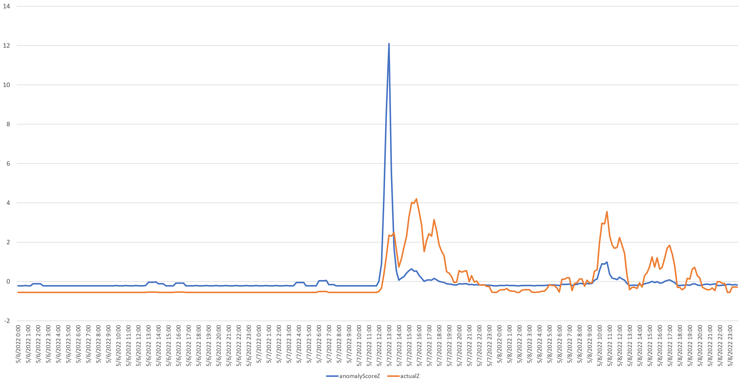
Since the API outputs the highest anomalyScore for each time step, we can plot these scores over time to visualize the strongest anomaly the API detected at each timestep.
The timeline below plots the Z-scores (standard deviations from the mean) of the number of mentions of monkeypox monitored by GDELT (in orange) against the Timeseries Insights API's maximum anomalyScore for the hour-long period preceding that moment in 15 minute increments from May 6 to 8, 2022. The two variables have very different vertical scales so they have been converted to Z-scores to make their relative changes more visible on the same Y axis.
Immediately clear is the massive vertical surge of the API's anomaly score right at the very beginning of the surge in mentions.
The timeline below zooms into this period, from 11AM UTC to 16:45PM UTC, showing the max anomaly score rising in lockstep with the initial surge of article mentions. Instead of Z scores, this displays their actual values. In fact, if you look closely you will see that the first two mentions occur at 12:00 UTC, with the API assigning an anomaly score of 1.3 (low strength) at that exact moment of 12:00UTC, while at 12:15 UTC with 10 mentions, the score rises to 6.59 ("very high" strength). This shows how responsive the API is in this configuration, alerting instantly to the earliest glimmers of media reporting on the outbreak.
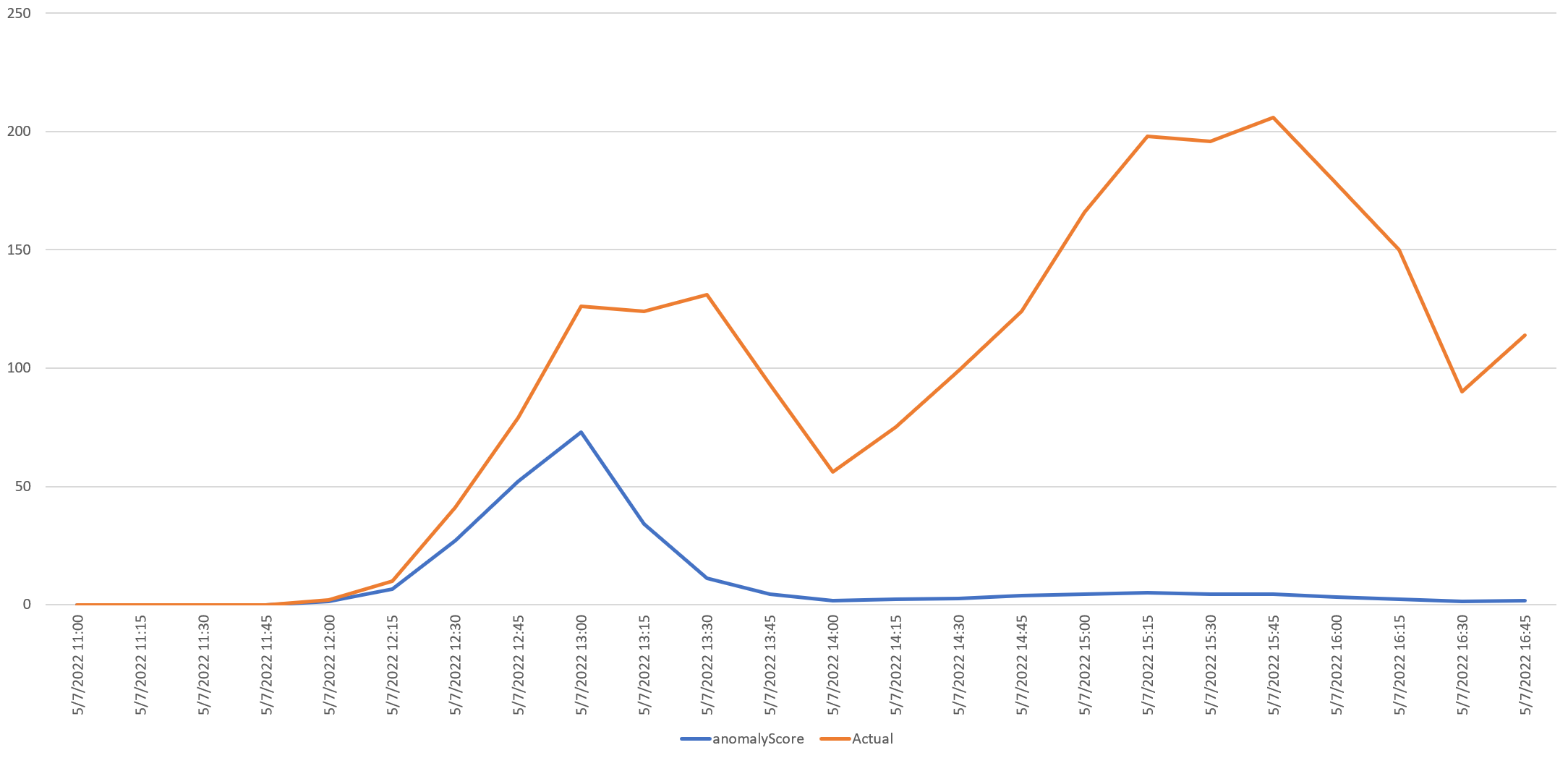
You can see the table underlying the graph below, showing how immediately responsive the API is using our query parameters, picking up the increasing mentions instantly and tapering off rapidly as the surge in mentions is no longer anomalous under our query conditions:
| anomalyScore | Mentions | |
| 5/7/2022 11:00 | 0 | 0 |
| 5/7/2022 11:15 | 0 | 0 |
| 5/7/2022 11:30 | 0 | 0 |
| 5/7/2022 11:45 | 0 | 0 |
| 5/7/2022 12:00 | 1.318915147 | 2 |
| 5/7/2022 12:15 | 6.594575734 | 10 |
| 5/7/2022 12:30 | 27.03776051 | 41 |
| 5/7/2022 12:45 | 52.0971483 | 79 |
| 5/7/2022 13:00 | 72.8198793 | 126 |
| 5/7/2022 13:15 | 34.13042224 | 124 |
| 5/7/2022 13:30 | 11.29432824 | 131 |
| 5/7/2022 13:45 | 4.344931919 | 93 |
| 5/7/2022 14:00 | 1.669585666 | 56 |
| 5/7/2022 14:15 | 2.264167566 | 75 |
| 5/7/2022 14:30 | 2.71636736 | 99 |
| 5/7/2022 14:45 | 3.815550736 | 124 |
| 5/7/2022 15:00 | 4.514502952 | 166 |
| 5/7/2022 15:15 | 5.111147594 | 198 |
| 5/7/2022 15:30 | 4.361877889 | 196 |
| 5/7/2022 15:45 | 4.460250498 | 206 |
| 5/7/2022 16:00 | 3.138049954 | 178 |
| 5/7/2022 16:15 | 2.328895961 | 150 |
| 5/7/2022 16:30 | 1.326171229 | 90 |
| 5/7/2022 16:45 | 1.619239731 | 114 |
Critically, there is no temporal lag, they move in perfect lockstep. As expected, the anomaly score begins climbing more slowly as article mentions continue to surge, then peaks and begins declining rapidly before leveling off back at a much lower score. This is because while mentions continue to surge, they are no longer anomalous under our query criteria (a rolling 1 hour window compared with the preceding 3 days). In an early warning sudden onset monitoring application it is this initial surge we typically wish to alert on, not the subsequent oscillation in mentions as the rest of the world begins to cover and contextualize the story – by that point we want to focus our alerting on the myriad other stories that are being drowned out by the initial story.
Of course, if we wanted to catch those secondary rises such as begins at 14:00 UTC, we could use a smaller rolling window and a larger time horizon. In other words, by tuning our query parameters we can ask the API to return any kind of anomaly of interest.
Looking at the May 6-8 timeline, we can see how the anomaly score rises again on May 8th as mentions again surge after a period of decreased mentions, showing how the API under our query configuration surfaces sudden surges after periods of quiet and then filters out continued increases. Simply by adjusting our query parameters we can change this behavior to flag any kind of anomalous behavior of interest.
In fact, a typical use case might involve running multiple queries every 15 minutes searching for different kinds of anomalies. One query might search for sudden onset surges like we've used in the example here. Another might use a longer time horizon to identify slow steady increases or decreases in mentions. Another might look only for lengthy increases of longer than a certain duration and so on. All of these queries can be run in parallel every 15 minutes, covering all anomaly types relevant to a specific use case. With the addition of contextual data to the timeseries, such as associated location, we could compute per-country or even per-city anomaly scores, creating a live-updating heatmap of the world.
Conclusion
We've shown how to use Translate API to quickly bootstrap a multilingual search, BigQuery to apply that search to GDELT's vast realtime planetary-scale archives and the Timeseries Insights API to perform realtime anomaly detection.
While the example here uses a static dataset, the Timeseries APIs' realtime append capability means the underlying dataset can trivially be updated in realtime, allowing you to use this exact workflow to perform true realtime horizon scanning.
Of course, the real power of the Timeseries API lies in its ability to identify anomalies at extreme scale. Rather than comparing the past hour against the past three days with a relatively small dataset like mentions of monkeypox, you could load the entire Web NGrams dataset into the API and compare today's mentions against the past several years, performing anomaly detection over extreme timeseries datasets with ease.
Using the same workflow we've presented here, you could expand the list of monitored topics to include a catalog of all known infectious diseases and trivially surface any anomalous increases or decreases in discussion of any of them and even map their scores by city or country. Since we encode each mention as its own groupId, you could add in the surrounding keywords in the pre and post KWIC snippet fields from the Web NGrams dataset and group them under the same groupId as the ngram. Using the Global Entity Graph, Global Geographic Graph, Global Embedded Metadata Graph and other GDELT datasets, a wealth of additional contextual features can be added. This would enable anomaly detection to be restricted by geographic area, just from certain outlets or languages, only those mentions in context with certain entities or surrounding terms, etc. For example, a common disease term could be filtered to only assess anomalous coverage trends of its appearance alongside words like "deaths" to only identify coverage of deaths related to the disease.
In the end, by pairing GDELT's Web NGrams 3.0 dataset with GCP's Timeseries Insights API, Translate API and BigQuery, we've created a realtime planetary-scale anomaly detection system for disease early warning and horizon scanning that scours global media for the intensity of discussion around any topic and flags anomalous changes in discussion, with the ability to fine-tune the system to precisely define the kind of anomaly of interest.