Last year BBVA showcased creating a global network of countries co-occurring in coverage relating to trade wars. Such powerful visualizations allow analysts to peer into the hidden geographic and network patterns embodied in global news coverage. Traditionally, constructing such visualizations required a considerable amount of work from the data analyst, though in 2015 we showcased how a single query in BigQuery, coupled with a lookup file, a PERL script and some additional work could streamline the creation of such visualizations.
Today we're excited to showcase a new pair of queries that perform the entire analysis entirely inside of BigQuery, outputting two files – one a node list and one an edge list, that can be saved and loaded directly into Gephi and visualized with just a few additional mouseclicks. In just 5 minutes, you can go from initial idea to final country co-occurrence network visualization!
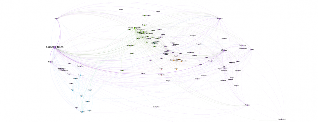
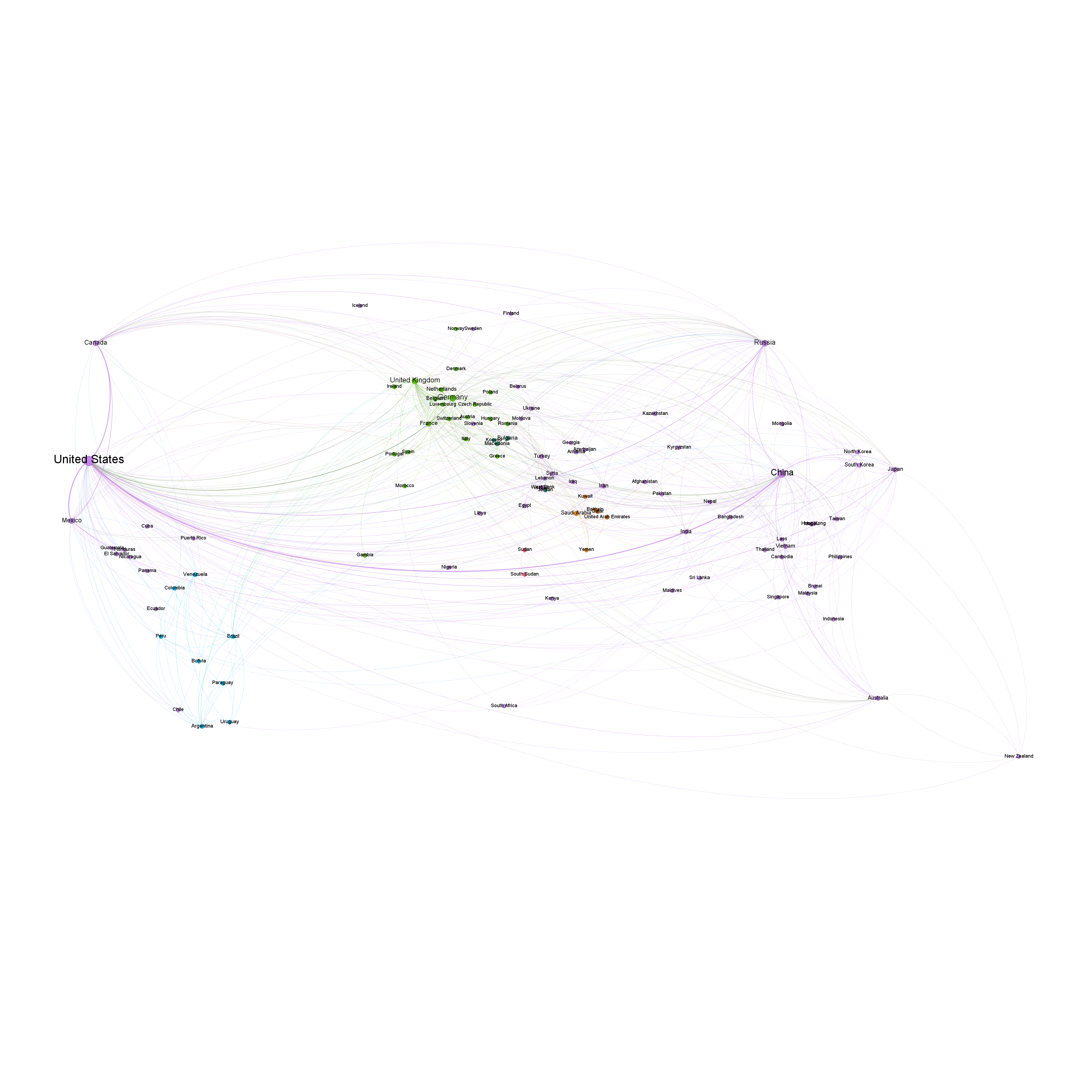
To demonstrate this new approach, let's say you want to visualize the countries most commonly mentioned together in worldwide coverage of "free trade" over the past four years. The GDELT Global Knowledge Graph (GKG) 2.0 has a built-in theme for this: "ECON_FREETRADE". To narrow our matches to articles that are actually about free trade rather than merely casually mentioning it off hand, we'll using the filter "where V2Themes like '%ECON_FREETRADE%ECON_FREETRADE%' " to require two or more mentions of free trade in the article.
Before we get to the details, here is the final network visualization so you can see the results! (There is also a transparent background version you can use with Photoshop/ImageMagick/etc to overlay onto your own static Mercator projection basemap – note that some browsers may display this as a black background when viewing in-browser but will display correctly when you download and view in Photoshop).

TECHNICAL DETAILS
We've adapted Felipe Hoffa's original BigQuery graph code to join against a country lookup file to convert the GKG's FIPs country codes to standardized human-friendly country names. This same lookup also contains the country centroids that we will use in a moment.
We've limited the graph to the top 500 strongest edges. Typically the top 500 edges in a country graph constitute the most meaningful edges and avoid saturating the graph with too many lines, but you can simply change the "limit 500" filter to any desired value. We also exclude "OS" matches which are world oceans, since the GKG's geocoder focuses on land-based locations and does not distinguish the individual oceans. The code below also includes a " DATE(_PARTITIONTIME) = "2019-11-10" " filter to restrict it to a single day to make it easier to experiment with. To run across the entire 4-year GKG, simply remove that line (though NOTE that that will typically consume 1.5TB or more of your monthly query quota).
The final edge table query is:
SELECT d.countryname Source, e.countryname Target, "Undirected" Type, ( c.Count/SUM(c.Count) OVER () ) Weight FROM (
SELECT a.countrycode Source, b.countrycode Target, COUNT(*) as Count
FROM (
 (SELECT DocumentIdentifier url, REGEXP_EXTRACT(location,r'^.*?#.*?#(.*?)#') countrycode FROM `gdelt-bq.gdeltv2.gkg_partitioned`, UNNEST(SPLIT(V2Locations,';')) AS location WHERE length(V2Locations) > 3 AND V2Themes like '%ECON_FREETRADE%ECON_FREETRADE%' and DATE(_PARTITIONTIME) = "2019-11-10")
) a
JOIN (
 (SELECT DocumentIdentifier url, REGEXP_EXTRACT(location,r'^.*?#.*?#(.*?)#') countrycode FROM `gdelt-bq.gdeltv2.gkg_partitioned`, UNNEST(SPLIT(V2Locations,';')) AS location WHERE length(V2Locations) > 3 AND V2Themes like '%ECON_FREETRADE%ECON_FREETRADE%' and DATE(_PARTITIONTIME) = "2019-11-10")
) b
ON a.url=b.url
WHERE a.countrycode<b.countrycode and a.countrycode != 'OS' and b.countrycode != 'OS'
GROUP BY 1,2
ORDER BY 3 DESC
LIMIT 500
) c
JOIN (
select fips, countryname from `gdelt-bq.extra.countrygeolookup`) d
ON c.Source = d.fips
JOIN (
select fips, countryname from `gdelt-bq.extra.countrygeolookup`) e
ON c.Target = e.fips
order by Count Desc
When run without the date restricters, this query takes just 2.5 minutes to complete.
Save the results of this query to a CSV file called "edges.csv".
Now run the corresponding query to construct the node list. This repeats the query above and then compiles the results into a list of unique nodes and adds in their centroid latitude and longitude coordinates. Why do we recompute the entire cooccurrence graph instead of just histogramming the country codes? The reason is that for a given graph it is likely that not all 281 countries identified by the GKG's geocoder will be present in a given graph. Depending on the specific query and the "limit" parameter used, a much smaller number of countries may be represented in the graph, which can only be identified by recomputing the graph – including the other countries would result in a perimeter of isolates surrounding a graph.
Thus, the final node list query becomes:
select Country Id, Country Label, Latitude, Longitude from (
WITH network AS(
SELECT d.countryname Source, d.latitude SourceLatitude, d.longitude SourceLongitude, e.countryname Target, e.latitude TargetLatitude, e.longitude TargetLongitude FROM (
SELECT a.countrycode Source, b.countrycode Target, COUNT(*) as Count
FROM (
 (SELECT DocumentIdentifier url, REGEXP_EXTRACT(location,r'^.*?#.*?#(.*?)#') countrycode FROM `gdelt-bq.gdeltv2.gkg_partitioned`, UNNEST(SPLIT(V2Locations,';')) AS location WHERE length(V2Locations) > 3 AND V2Themes like '%ECON_FREETRADE%ECON_FREETRADE%' and DATE(_PARTITIONTIME) = "2019-11-10")
) a
JOIN (
 (SELECT DocumentIdentifier url, REGEXP_EXTRACT(location,r'^.*?#.*?#(.*?)#') countrycode FROM `gdelt-bq.gdeltv2.gkg_partitioned`, UNNEST(SPLIT(V2Locations,';')) AS location WHERE length(V2Locations) > 3 AND V2Themes like '%ECON_FREETRADE%ECON_FREETRADE%' and DATE(_PARTITIONTIME) = "2019-11-10")
) b
ON a.url=b.url
WHERE a.countrycode<b.countrycode and a.countrycode != 'OS' and b.countrycode != 'OS'
GROUP BY 1,2
ORDER BY 3 DESC
LIMIT 500
) c
JOIN (
select fips, countryname, latitude, longitude from `gdelt-bq.extra.countrygeolookup`) d
ON c.Source = d.fips
JOIN (
select fips, countryname, latitude, longitude from `gdelt-bq.extra.countrygeolookup`) e
ON c.Target = e.fips
order by Count Desc
)
( select Source Country, SourceLatitude Latitude, SourceLongitude Longitude from network )
UNION DISTINCT
( select Target Country, TargetLatitude Latitude, TargetLongitude Longitude from network )
) order by Country
Save the results of this query to a CSV file and name it "nodes.csv".
Now open Gephi and install the "geolayout" plugin using Gephi's plugin manager. Then create a new project, go to the Data Laboratory tab, click on the "Import Spreadsheet" button and load the "nodes.csv" file (making sure in the import wizard to select that it is a "node list") and making sure that you select "append to current workspace" rather than "create new workspace".
Then click on the "Import Spreadsheet" button again and load the "edges.csv" file (making sure this time in the import wizard to select that it is an "edge list") and making sure that you select "append to current workspace" rather than "create new workspace".
The order of these two steps does not matter in current versions of Gephi – you can import the edges file and then the nodes file or vice-versa. The most important step is that you correctly select whether it is an "edge list" or "node list" and that you select "append to current workspace" on the final screen of the import wizard before clicking on the "Finish" button (the default is "create new workspace"). If you find that you are missing lat/long coordinates, you likely forgot to click the "append" option.
Finally, back under the "Overview" tab go to the layout algorithms, click "Geo Layout" and click the run button to instantly snap the country nodes to their proper locations. You can also adjust the projection depending on preference and/or if you plan to export as a transparent image and overlay onto a static basemap using Photoshop/ImageMagick/etc.
The graphs above were colored using Modularity with node size according to PageRank.
Happy geographic network visualizing!