
Making the GDELT Global Knowledge Graph available in Google BigQuery has been one of the most-requested features since the debut of the GDELT Event archive in BigQuery last May. Now that GKG 2.0 is available in BigQuery as part of GDELT 2.0, we've been hearing from many of you asking for help in working with the GKG's complex multi-delimiter fields using SQL so that you can perform your analyses entirely in BigQuery without having to do any final parsing or histogramming in a scripting language like PERL or Python.
With the expert help of Felipe Hoffa, Developer Advocate on big data at Google, we've put together a set of example queries that show how to use some of the more advanced string manipulation features of BigQuery to parse the delimited fields in the GKG and generate various kinds of histograms. With just a single line of SQL, you can now use BigQuery to perform arbitrarily-complex queries on the GKG, parse the delimited results, convert them into a histogram, and deliver the final results downloadable as a spreadsheet!
Once you've created a Google BigQuery account, browse on over to the GKG table in BigQuery, click on the "Query Table" button towards the top right of the screen, and follow along with the examples below!
PERSON/ORGANIZATION/THEME HISTOGRAMS
Often you want to be able to run a query on the GKG and get back a list of the top people, organizations, general names, or themes that appear in matching coverage. For example, imagine creating a histogram of the top themes associated with Israeli Prime Minister Benjamin Netanyahu during his visit to the US Congress on March 3, 2015.
Requesting a list of the themes appearing in each article mentioning his name is trivial to do in BigQuery:
SELECT V2Themes from [gdelt-bq:gdeltv2.gkg] where DATE>20150302000000 and DATE < 20150304000000 and V2Persons like '%Netanyahu%' limit 10;
The problem is that the resulting rows look like:
TAX_FNCACT_SUPPORTERS,1512;TAX_POLITICAL_PARTY_REPUBLICANS,691;TERROR,1844;ARMEDCONFLICT,1844;TAX_FNCACT_LEADERS,1647;TAX_FNCACT_LEADERS,1716;LEADER,85;LEADER,2189;TAX_FNCACT_PRIME_MINISTER,85;TAX_FNCACT_PRIME_MINISTER,2189;TAX_FNCACT_LEADER,911;WMD,1112;TAX_FNCACT_PRESIDENT,800;TAX_FNCACT_PRESIDENT,1362;
The issue is that the V2Themes column uses nested delimiting – each mention of a recognized theme in an article is separated by a semicolon, and for each mention, the theme and its character offset within the article are separated by a comma. How can we ask BigQuery to split up the V2Themes field from each matching record and, at the same time, split off the ",character offset" from the end of each theme mention?
First, we use the SPLIT() function to tell BigQuery to take the V2Themes field and break it up by semicolon and return it as multiple records, one per mention. In other words, using "SPLIT(V2Themes,
TAX_FNCACT_SUPPORTERS,1512
TAX_POLITICAL_PARTY_REPUBLICANS,691
TERROR,1844
ARMEDCONFLICT,1844
TAX_FNCACT_LEADERS,1647
TAX_FNCACT_LEADERS,1716
LEADER,85
LEADER,2189
TAX_FNCACT_PRIME_MINISTER,85
TAX_FNCACT_PRIME_MINISTER,2189
TAX_FNCACT_LEADER,911
WMD,1112
TAX_FNCACT_PRESIDENT,800
TAX_FNCACT_PRESIDENT,1362
Note how it has also helpfully unrolled each mention into its own returned record. The problem is that we still have the character offset listed at the end of each theme mention that we need to get rid of. To assist with this, BigQuery has the helpful REGEXP_REPLACE() function – we can write an arbitrary regular expression to rewrite any field as needed. In this case, we combine the SPLIT() and REGEXP_REPLACE() functions together, to get "REGEXP_REPLACE(SPLIT(AllNames,
The final query that puts all of this together and returns the top 300 themes from all coverage of Netanyahu's visit is:
FROM (
select REGEXP_REPLACE(SPLIT(V2Themes,';'), r',.*', ") theme
from [gdelt-bq:gdeltv2.gkg]
where DATE>20150302000000 and DATE < 20150304000000 and V2Persons like '%Netanyahu%'
)
group by theme
ORDER BY 2 DESC
LIMIT 300
If you look at the results, they make a lot of sense (note the appearance of a number of World Bank Topical Taxonomy headings):
| Row | theme | count | |
| 1 | GENERAL_GOVERNMENT | 33677 | |
| 2 | LEADER | 33405 | |
| 3 | TAX_FNCACT_MINISTER | 31174 | |
| 4 | TAX_FNCACT_PRESIDENT | 25981 | |
| 5 | TAX_FNCACT_PRIME_MINISTER | 25560 | |
| 6 | WB_2432_FRAGILITY_CONFLICT_AND_VIOLENCE | 14865 | |
| 7 | WB_696_PUBLIC_SECTOR_MANAGEMENT | 13797 | |
| 8 | NEGOTIATIONS | 13567 | |
| 9 | WB_2470_PEACE_OPERATIONS_AND_CONFLICT_MANAGEMENT | 13508 | |
| 10 | WB_840_JUSTICE | 13390 | |
| 11 | WB_936_ALTERNATIVE_DISPUTE_RESOLUTION | 13009 | |
| 12 | WB_843_DISPUTE_RESOLUTION | 13009 | |
| 13 | WB_2471_PEACEKEEPING | 12883 | |
| 14 | WB_2473_DIPLOMACY_AND_NEGOTIATIONS | 12841 |
Now, let's compare these results against those for Greek Prime Minister Alexis Tsipras during the same period:
FROM (
select REGEXP_REPLACE(SPLIT(V2Themes,';'), r',.*', ") theme
from [gdelt-bq:gdeltv2.gkg]
where DATE>20150302000000 and DATE < 20150304000000 and V2Persons like '%Tsipras%'
)
group by theme
ORDER BY 2 DESC
LIMIT 300
As expected, we see a very different set of topc themes, which strongly reflect Greece's economic and debt-related discourse:
| Row | theme | count | |
| 1 | GENERAL_GOVERNMENT | 5502 | |
| 2 | TAX_FNCACT_MINISTER | 5184 | |
| 3 | TAX_WORLDLANGUAGES_GREEK | 4251 | |
| 4 | TAX_ETHNICITY_GREEK | 4205 | |
| 5 | ECON_BANKRUPTCY | 3514 | |
| 6 | LEADER | 2743 | |
| 7 | TAX_FNCACT_PRIME_MINISTER | 2286 | |
| 8 | ECON_WORLDCURRENCIES_EURO | 1036 | |
| 9 | NEGOTIATIONS | 1030 | |
| 10 | WB_696_PUBLIC_SECTOR_MANAGEMENT | 1013 | |
| 11 | TAX_ETHNICITY_SPANISH | 958 | |
| 12 | ELECTION | 957 | |
| 13 | TAX_WORLDLANGUAGES_SPANISH | 952 | |
| 14 | WB_1104_MACROECONOMIC_VULNERABILITY_AND_DEBT | 915 |
Finally, it is important to note that the query above counts every mention of each theme – if a theme is mentioned 100 times in a single article, it will count as much as a theme that is mentioned once in each of 100 different articles. Often this is the desired behavior, but if you would like to change this to count the number of documents mentioning a theme, rather than the number of mentions of a theme (ie, a theme that appears 100 times in a single article is only counted as one "appearance"), then you can simply wrap the REGEXP_REPLACE(SPLIT()) in a UNIQUE() call like the following:
FROM (
select UNIQUE(REGEXP_REPLACE(SPLIT(V2Themes,';'), r',.*', ")) theme
from [gdelt-bq:gdeltv2.gkg]
where DATE>20150302000000 and DATE < 20150304000000 and V2Persons like '%Netanyahu%'
)
group by theme
ORDER BY 2 DESC
LIMIT 300
This subtly changes the results to emphasize certain topics and de-emphasize others.
| Row | theme | count | |
| 1 | LEADER | 12807 | |
| 2 | GENERAL_GOVERNMENT | 11520 | |
| 3 | TAX_FNCACT_MINISTER | 11267 | |
| 4 | TAX_FNCACT_PRIME_MINISTER | 10244 | |
| 5 | TAX_FNCACT_PRESIDENT | 9382 | |
| 6 | WB_2432_FRAGILITY_CONFLICT_AND_VIOLENCE | 8853 | |
| 7 | WB_2470_PEACE_OPERATIONS_AND_CONFLICT_MANAGEMENT | 7814 | |
| 8 | NEGOTIATIONS | 7449 | |
| 9 | WMD | 7320 | |
| 10 | WB_696_PUBLIC_SECTOR_MANAGEMENT | 7249 | |
| 11 | WB_2471_PEACEKEEPING | 6868 | |
| 12 | WB_840_JUSTICE | 6851 | |
| 13 | WB_2473_DIPLOMACY_AND_NEGOTIATIONS | 6831 | |
| 14 | WB_936_ALTERNATIVE_DISPUTE_RESOLUTION | 6511 |
This approach can also be applied to the V2Persons, V2Organizations, and AllNames fields. For example, the following query returns those person names mentioned in the most articles about Prime Minister Netanyahu's visit to the US by just changing the SPLIT() function to use the "V2Persons" field instead of "V2Themes":
SELECT person, COUNT(*) as count
FROM (
select UNIQUE(REGEXP_REPLACE(SPLIT(V2Persons,';'), r',.*', ")) person
from [gdelt-bq:gdeltv2.gkg]
where DATE>20150302000000 and DATE < 20150304000000 and V2Persons like '%Netanyahu%'
)
group by person
ORDER BY 2 DESC
LIMIT 300
The substantial references to Winston Churchill are intriguing:
| Row | person | count | |
| 1 | Benjamin Netanyahu | 12995 | |
| 2 | Barack Obama | 6391 | |
| 3 | John Kerry | 4434 | |
| 4 | John Boehner | 4176 | |
| 5 | Joe Biden | 1705 | |
| 6 | Mohammad Javad Zarif | 1585 | |
| 7 | Nancy Pelosi | 785 | |
| 8 | Winston Churchill | 732 | |
| 9 | Elie Wiesel | 576 | |
| 10 | Isaac Herzog | 323 | |
| 11 | Matthew Lee | 318 | |
| 12 | Barak Obama | 314 | |
| 13 | Valerie Jarrett | 270 | |
| 14 | Mohammed Javad Zarif | 247 |
Finally, you can also use this approach to topically characterize entire outlets:
select SourceCommonName, theme, count from (
SELECT SourceCommonName, theme, COUNT(*) as count
FROM (
select SourceCommonName, UNIQUE(REGEXP_REPLACE(SPLIT(V2Themes,';'), r',.*', ")) theme
from [gdelt-bq:gdeltv2.gkg] where DATE >= 20150200000000 AND DATE< 20151099999999
)
group by SourceCommonName, theme
) where count > 100
ORDER BY count DESC
COMPARING LANGUAGES
Often it is useful to compare how a situation is being contextualized differently across languages. Recall that GDELT 2.0 now live-translates the world's news in 65 languages in realtime. We can use the "TranslationInfo" field to compare the topical focus of Hebrew vs Arabic-language coverage of Netanyahu's visit.
The query below repeats the topical histogram query of earlier, but this time adds an additional filter to the WHERE clause to restrict the results to only Hebrew-language news coverage:
SELECT theme, COUNT(*) as count
FROM (
select UNIQUE(REGEXP_REPLACE(SPLIT(V2Themes,';'), r',.*', ")) theme
from [gdelt-bq:gdeltv2.gkg]
where DATE>20150302000000 and DATE < 20150304000000 and AllNames like '%Netanyahu%' and TranslationInfo like '%srclc:heb%'
)
group by theme
ORDER BY 2 DESC
LIMIT 300
This generates the following themes, focused primarily on political violence, conflict, the Palestinians, but also, of particular interest with the upcoming Israeli elections, domestic issues such as unemployment:
LEADER
ARMEDCONFLICT
TAX_RELIGION_JEWS
WB_2462_POLITICAL_VIOLENCE_AND_WAR
WB_2432_FRAGILITY_CONFLICT_AND_VIOLENCE
TAX_FNCACT_MINISTER
TAX_ETHNICITY_ARAB
TAX_FNCACT_PRIME_MINISTER
WB_2433_CONFLICT_AND_VIOLENCE
ELECTION
TAX_ETHNICITY_PALESTINIANS
TAX_FNCACT_POLICE
SECURITY_SERVICES
WB_2670_JOBS
TAX_FNCACT_SOLDIERS
WB_2747_UNEMPLOYMENT
TAX_RELIGION_JEW
TAX_POLITICAL_PARTY_LIKUD
TAX_RELIGION_JEWISH
WB_739_POLITICAL_VIOLENCE_AND_CIVIL_WAR
Now, let's repeat this query, but this time for Arabic-language coverage:
SELECT theme, COUNT(*) as count
FROM (
select UNIQUE(REGEXP_REPLACE(SPLIT(V2Themes,';'), r',.*', ")) theme
from [gdelt-bq:gdeltv2.gkg]
where DATE>20150302000000 and DATE < 20150304000000 and AllNames like '%Netanyahu%' and TranslationInfo like '%srclc:ara%'
)
group by theme
ORDER BY 2 DESC
LIMIT 300
The resulting thematic breakdown paints a very different picture of reaction to his visit to the US:
GENERAL_GOVERNMENT
LEADER
TAX_FNCACT_PRESIDENT
WB_2432_FRAGILITY_CONFLICT_AND_VIOLENCE
TAX_ETHNICITY_IRANIAN
WB_696_PUBLIC_SECTOR_MANAGEMENT
WB_840_JUSTICE
NEGOTIATIONS
WB_2470_PEACE_OPERATIONS_AND_CONFLICT_MANAGEMENT
WB_2471_PEACEKEEPING
WB_843_DISPUTE_RESOLUTION
WB_936_ALTERNATIVE_DISPUTE_RESOLUTION
WB_2473_DIPLOMACY_AND_NEGOTIATIONS
WB_939_NEGOTIATION
TAX_FNCACT_MINISTER
MEDIA_MSM
WMD
ELECTION
TAX_FNCACT_FOREIGN_MINISTER
ARMEDCONFLICT
Arabic-language coverage of his visit seems to be much more strongly focused on dispute resolution and diplomatic negotiations, with far less coverage of political violence and conflict.
Of course, comparing topical breakdowns across languages requires a lot of careful consideration regarding possible differences in language and narrative (for example discussion of "Iran the country" versus "Iranians the people"), which can affect which themes are triggered and even complexities in how certain topics may or may not map ideally into each language. At the very least, however, such comparisons can provide very useful unexpected patterns or results for further human investigation.
GEOGRAPHIC HISTOGRAMS
Creating geographic histograms using the V2Locations field is more complex than the other fields due to the larger number of attributes recorded for each location and the additional need for certain queries to filter by those attributes. Creating histograms of the geographic fields requires more extensive use of BigQuery's regular expression capabilities, especially its REGEXP_EXTRACT() function, which allows the use of regular expressions to extract information from a field as part of a SELECT(). BigQuery's regular expression syntax supports incredibly powerful queries, though it does not support all of the capability of PERL or similar regular expressions.
Per the GKG 2.0 file format documentation, the format of the V2Location field is semicolon delimited (each mention of a location is separated by a semicolon), with the details of each location mention separated by the pound symbol ("#"). For each location mention, the details recorded (in order of appearance) are:
- Location Type. (integer) This field specifies the geographic resolution of the match type and holds one of the following values: 1=COUNTRY (match was at the country level), 2=USSTATE (match was to a US state), 3=USCITY (match was to a US city or landmark), 4=WORLDCITY (match was to a city or landmark outside the US), 5=WORLDSTATE (match was to an Administrative Division 1 outside the US – roughly equivalent to a US state). This can be used to filter counts by geographic specificity, for example, extracting only those counts with a landmark-level geographic resolution for mapping. Note that matches with codes 1 (COUNTRY), 2 (USSTATE), and 5 (WORLDSTATE) will still provide a latitude/longitude pair, which will be the centroid of that country or state, but the FeatureID field below will contain its textual country or ADM1 code instead of a numeric featureid.
- Location FullName. (text) This is the full human-readable name of the matched location. In the case of a country it is simply the country name. For US and World states it is in the format of “State, Country Name”, while for all other matches it is in the format of “City/Landmark, State, Country”. This can be used to label locations when placing counts on a map. Note: this field reflects the precise name used to refer to the location in the text itself, meaning it may contain multiple spellings of the same location – use the FeatureID column to determine whether two location names refer to the same place.
- Location CountryCode. (text) This is the 2-character FIPS10-4 country code for the location. Note: GDELT continues to use the FIPS10-4 codes under USG guidance while GNS continues its formal transition to the successor Geopolitical Entities, Names, and Codes (GENC) Standard (the US Government profile of ISO 3166). Note that from 2/19/2015 through midday 3/1/2015 there was an error that affected some records, causing them to have an invalid value in this field.
- Location ADM1Code. (text) This is the 2-character FIPS10-4 country code followed by the 2-character FIPS10-4 administrative division 1 (ADM1) code for the administrative division housing the landmark. In the case of the United States, this is the 2-character shortform of the state’s name (such as “TX” for Texas). Note: see the notice above for CountryCode regarding the FIPS10-4 / GENC transition.
- Location ADM2Code (integer). This is is the numeric GAUL code for the administrative division 2 (ADM2) for the administrative division housing the landmark (if available). For more details on this field, please see the following announcement.
- Location Latitude. (floating point number) This is the centroid latitude of the landmark for mapping. In the case of a country or administrative division this will reflect the centroid of that entire country/division.
- Location Longitude. (floating point number) This is the centroid longitude of the landmark for mapping. In the case of a country or administrative division this will reflect the centroid of that entire country/division.
- Location FeatureID. (text OR signed integer) This is the numeric GNS or GNIS FeatureID for this location OR a textual country or ADM1 code. More information on these values can be found in Leetaru (2012).4 Note: This field will be blank or contain a textual ADM1 code for country or ADM1-level matches – see above. Note: For numeric GNS or GNIS FeatureIDs, this field can contain both positive and negative numbers, see Leetaru (2012) for more information on this.
- Character Offset. (integer) This is the approximate character offset within the document where the location was mentioned.
Thus, a typical entry might look like "4#Berlin, Berlin, Germany#GM#GM16#16538#52.5167#13.4#-1746443#1340", indicating a reference to Berlin, Germany.
To start things off, here is a simple query that returns a histogram of locations mentioned in coverage of Greek Prime Minister Tsipras during the same period as the theme query from earlier:
SELECT location, COUNT(*)
FROM (
select REGEXP_EXTRACT(SPLIT(V2Locations,';'),r'^.*?#(.*?)#') as location
from [gdelt-bq:gdeltv2.gkg]
where DATE>20150302000000 and DATE < 20150304000000 and V2Persons like '%Tsipras%'
)
group by location
ORDER BY 2 DESC
LIMIT 100
As might be expected, many of the top results are country-level locations like "Greece" and "Spain", which are likely of less interest for many queries. Instead, the following query modifies the REGEXP_EXTRACT slightly to add "[2-5]" at the start of the query instead of the original ".*?" (filtering each location mention to require a value between 2 and 5 for the "Location Type" field (anything higher-resolution than a country-level match).
SELECT location, COUNT(*)
FROM (
select REGEXP_EXTRACT(SPLIT(V2Locations,';'),r'^[2-5]#(.*?)#') as location
from [gdelt-bq:gdeltv2.gkg]
where DATE>20150302000000 and DATE < 20150304000000 and V2Persons like '%Tsipras%'
)
where location is not null
group by location
ORDER BY 2 DESC
LIMIT 100
Of course, not all of those results are in Greece, so by adding an additional filter to also require "GR" (the country code for Greece) in the "Location CountryCode" field, the following query returns a histogram of all city-level locations in Greece mentioned in coverage of the Prime Minister:
SELECT location, COUNT(*)
FROM (
select REGEXP_EXTRACT(SPLIT(V2Locations,';'),r'^[2-5]#(.*?)#GR#') as location
from [gdelt-bq:gdeltv2.gkg]
where DATE>20150302000000 and DATE < 20150304000000 and V2Persons like '%Tsipras%'
)
where location is not null
group by location
ORDER BY 2 DESC
LIMIT 100
The following query expands this a bit, allowing city-level matches from Greece ("GR"), Germany ("GM") and Spain ("SP"), using a "non-capture group" in the regular expression:
SELECT location, COUNT(*)
FROM (
select REGEXP_EXTRACT(SPLIT(V2Locations,';'),r'^[2-5]#(.*?)#(?:GR|GM|SP)#') as location
from [gdelt-bq:gdeltv2.gkg]
where DATE>20150302000000 and DATE < 20150304000000 and V2Persons like '%Tsipras%'
)
where location is not null
group by location
ORDER BY 2 DESC
LIMIT 100
Finally, for mapping purposes, you might want to export just a latitude/longitude histogram to pass to a mapping program:
SELECT coord, COUNT(*)
FROM (
select REGEXP_REPLACE(REGEXP_EXTRACT(SPLIT(V2Locations,';'),r'^[2-5]#.*?#.*?#.*?#.*?#(.*?#.*?)#'), '^(.*?)#(.*?)', '\1;\2') as coord
from [gdelt-bq:gdeltv2.gkg]
where DATE>20150302000000 and DATE < 20150304000000 and V2Persons like '%Tsipras%'
)
where coord is not null
group by coord
ORDER BY 2 DESC
LIMIT 100
Finally, this query modifies the one above to add in the name of the city into each match by modifying the REGEXP_EXTRACT to return multiple attributes and then using REGEXP_REPLACE to parse them out into the final results (NOTE that in cases of highly geographically proximate features, or multiple alternative names for a given feature, the query below may yield multiple records with the same lat/long, but different names):
SELECT namedcoord, COUNT(*)
FROM (
select REGEXP_REPLACE(REGEXP_EXTRACT(SPLIT(V2Locations,';'),r'^[2-5]#(.*?#.*?#.*?#.*?#.*?#.*?)#'), '^(.*?)#.*?#.*?#.*?#(.*?)#(.*?)', '\1;\2;\3') as namedcoord
from [gdelt-bq:gdeltv2.gkg]
where DATE>20150302000000 and DATE < 20150304000000 and V2Persons like '%Tsipras%'
)
where namedcoord is not null
group by namedcoord
ORDER BY 2 DESC
LIMIT 100
NETWORK ANALYSIS
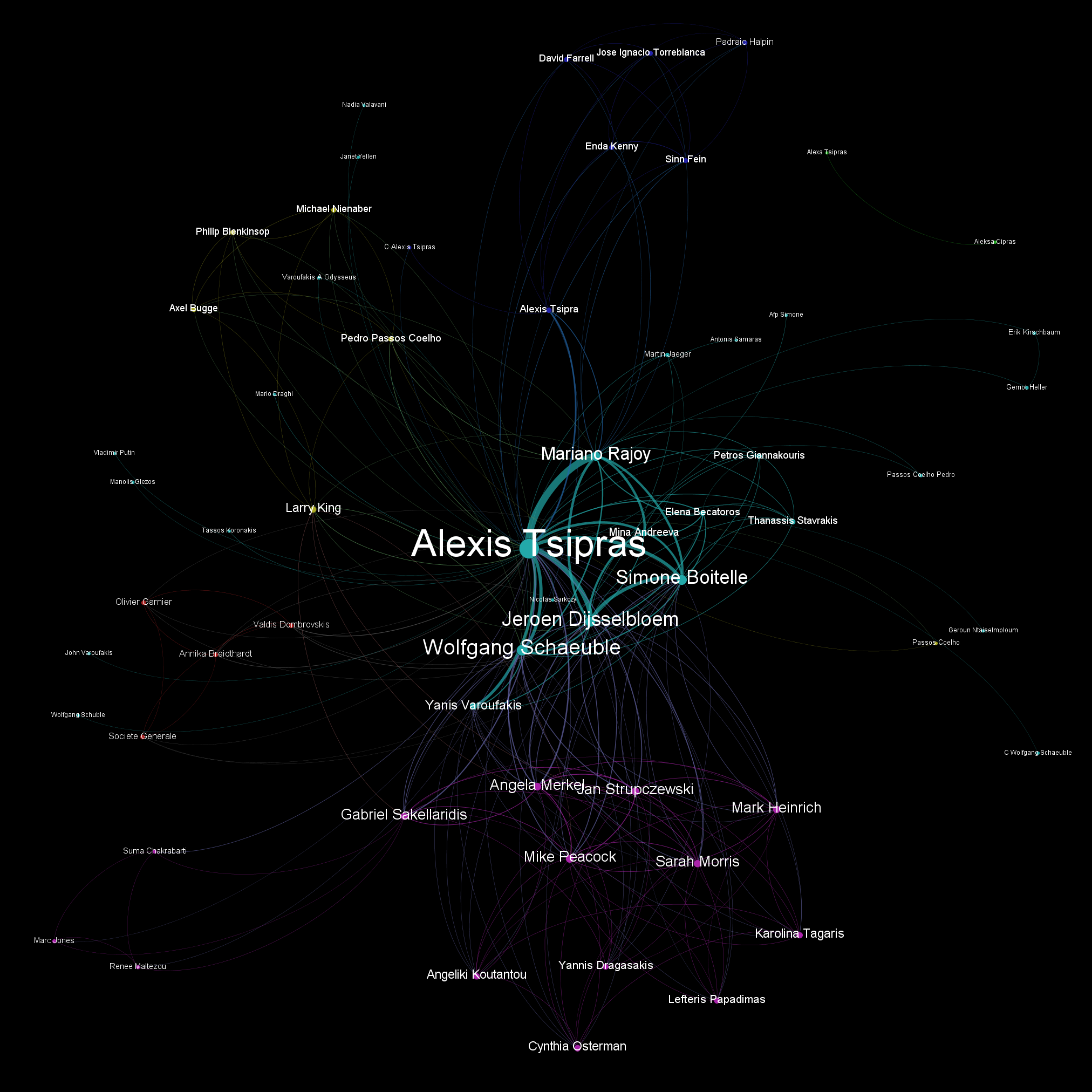
Finally, often it is the connections among entities that is of greatest interest, rather than just their frequency of occurrence. For example, what if you wanted to understand the web of connections surrounding Greek Prime Minister Alexis Tsipras, creating a network diagram showing all of the people he is most closely connected to in the press during a particular time period or in relation to a particular topic? The following query creates a cooccurence network diagram of the people appearing in coverage of Prime Minister Tsipras during the period March 2, 2015 to March 4, 2015:
SELECT a.name, b.name, COUNT(*) as count
FROM (FLATTEN(
SELECT GKGRECORDID, UNIQUE(REGEXP_REPLACE(SPLIT(V2Persons,';'), r',.*', ")) name
FROM [gdelt-bq:gdeltv2.gkg]
WHERE DATE>20150302000000 and DATE < 20150304000000 and V2Persons like '%Tsipras%'
,name)) a
JOIN EACH (
SELECT GKGRECORDID, UNIQUE(REGEXP_REPLACE(SPLIT(V2Persons,';'), r',.*', ")) name
FROM [gdelt-bq:gdeltv2.gkg]
WHERE DATE>20150302000000 and DATE < 20150304000000 and V2Persons like '%Tsipras%'
) b
ON a.GKGRECORDID=b.GKGRECORDID
WHERE a.name<b.name
GROUP EACH BY 1,2
ORDER BY 3 DESC
LIMIT 250
The query is a bit complex, but to modify it to generate a network of person names around any query of interest, just change the first two WHERE() clauses to your query of interest. Essentially what the query does is to compile the list of person names from each matching article and record how many articles each pair of names appear together anywhere in the article. The final results of the query is a histogram of all pairs of names and how many articles they appeared together – essentially the "edge list" of the cooccurance network of persons.
Once you run the query above in BigQuery, click on the "Download as CSV" button at the top right of the query results table. This will download a CSV file to your local computer containing the results. Open the file in Excel and rename the first column to be "Source", the second to be "Target". Create a new column called "Type" and fill it in as "Undirected" for every row. Create another new column and call it "Weight". Set it to be the formula "=C2/SUM(C:C)" and copy-paste to all rows so that the value of this column for each row is essentially its percent of the total of column C (the "count" column). Basically this converts the raw article count of the "counts" column into a floating point value from 0 to 1 that Gephi prefers. The spreadsheet should now look like:
| Source | Target | count | Type | Weight |
| Alexis Tsipras | Mariano Rajoy | 496 | Undirected | 0.056998 |
| Alexis Tsipras | Jeroen Dijsselbloem | 334 | Undirected | 0.038382 |
| Alexis Tsipras | Simone Boitelle | 229 | Undirected | 0.026316 |
| Jeroen Dijsselbloem | Simone Boitelle | 229 | Undirected | 0.026316 |
| Alexis Tsipras | Wolfgang Schaeuble | 221 | Undirected | 0.025396 |
| Alexis Tsipras | Yanis Varoufakis | 199 | Undirected | 0.022868 |
| Jeroen Dijsselbloem | Mariano Rajoy | 175 | Undirected | 0.02011 |
Finally, save the file somewhere on your computer where you can find it again in a moment.
Download a copy of the open source Gephi package and install it on your computer. Run Gephi and choose "New Project" from the "File" menu. Click on the "Data Laboratory" button in the top left right under the menu bar. At top left under the "Data Table" tab you should see a row of buttons – click on the "Import Spreadsheet" button and on the popup that appears browse for the spreadsheet you just saved. Under the "As table" dropdown on the popup, choose "Edges table". Then click the "Next" button on the popup. Then click the "Finish" button on the popup. You should now see a spreadsheet. Click on the "Nodes" button towards the top-left right under the "Data Table" tab (in the same row where you found "Import Spreadsheet"). At the bottom of the window, click on the "Copy data to other column" button and choose "ID". From the popup that appears, choose "Label" and click "OK". This tells Gephi to use the name of each node as its human-readable label.
Now click on the "Overview" button at the top-left of Gephi (immediately to the left of the "Data Laboratory" button you clicked earlier). On the right side of the screen, click on the "Run" button beside "Modularity" (about midway down the list in the tab on the right side of the screen). Click OK on the popup that appears and then Gephi will pause for a few moments, and then click "Close" on the next popup that appears. Now, on the left side of the screen, towards the top, you should see a "Partition" tab – click on it. Then click on the twin circular green arrows button (the refresh button). This will populate the dropdown to its right – choose "Modularity Class" from the dropdown. Then click the "Apply" button on the lower right of that tab. The nodes on the network should now be colored.
Now click on the "Ranking" tab right beside the "Partition" tab. Click on the little icon that looks like a red diamond (if you mouse over it it says "Size/Weight"). Choose "Degree" from the dropdown and set "Min size" to "7" and "Max size" to "40" and then click "Apply". The nodes should now be different sizes based on their importance in the network.
Now go down to the "Layout" tab (bottom half of the left side of the window) and choose "Force Atlas 2" from the dropdown. Then click on the "Run" button. Let it run for around 10-15 seconds or until it looks like it has unfolded into some kind of legible structure and click on the "Run" button again (it says "Stop" while it is running). Note that this is called "graph layout" and this algorithm will continue forever if left alone (it doesn't have an ending point), so you have to manually stop it once it looks "right".
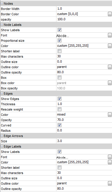
Now go back to the top of the window and click on the "Preview" button (to the right of the "Data Laboratory" button). On the left side there is a set of configuration options for the graph. Set them to be the following:
Now, finally, click on the "Refresh" button at the bottom left of the window. You should now see a network diagram that looks like the following (the colors and positions of nodes will be different each time you run Gephi, since it randomizes these). Congratulations, you have now visualized the co-occurance network of people co-occuring in coverage of the Prime Minister of Greece over a two day period! Looking through the network below the names most closely associated with the Prime Minister are those most closely involved in either Greece's negotiations with the EU or the related narrative surrounding Greece's debt restructuring and austerity discussions.
We hope that this has given you some ideas of how to leverage the enormous power of BigQuery to not only conduct realtime complex queries over the GDELT GKG, but to go much further, having BigQuery even parse and histogram the results for you, delivering the final analytic results. In this way, using the GKG with BigQuery is an example of loading massive CSV data into BigQuery to provide realtime analytics over highly structured flattened data. We'd like to thank Felipe Hoffa again for his tremendous help in navigating how to process the GKG's complex delimited structure into BigQuery's advanced string functions and in formulating and tuning these queries. We can't wait to see what you're able to accomplish!