In 2016 we visualized a year of the co-occurrence geography of the world's cities using a single line of SQL in BigQuery, courtesy of Felipe Hoffa. Last year we expanded this to visualize the geography of 2015-2018. We've repeated the analysis for 2015-2019, visualizing a total of  26.8 billion co-occurrences of 7.9 million distinct city pairings over nearly a billion articles. Again, just a single SQL query and 3.7 minutes was all it took to visualize it in BigQuery. The resulting graph was visualized using GraphViz.

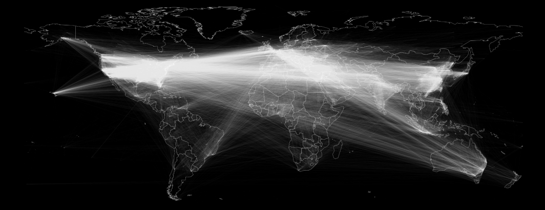
Using a cutoff of only pairings that appeared in at least 500 of the billion articles, the map below is so dense as to be almost meaningless, though it reminds us just how truly interconnected our world really is, in that every line below traces a pair of cities that were mentioned together more than 500 times over the last four years.

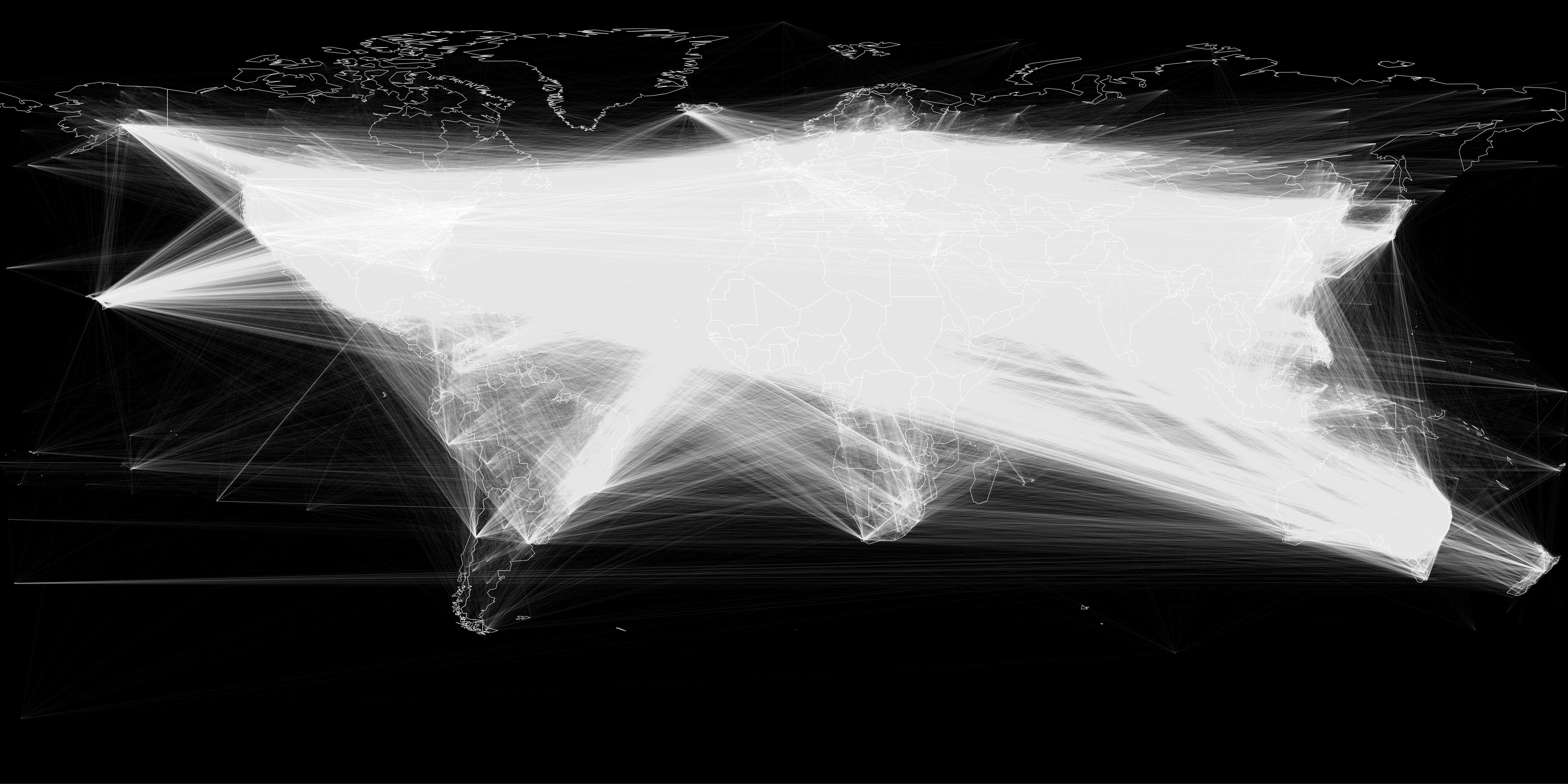
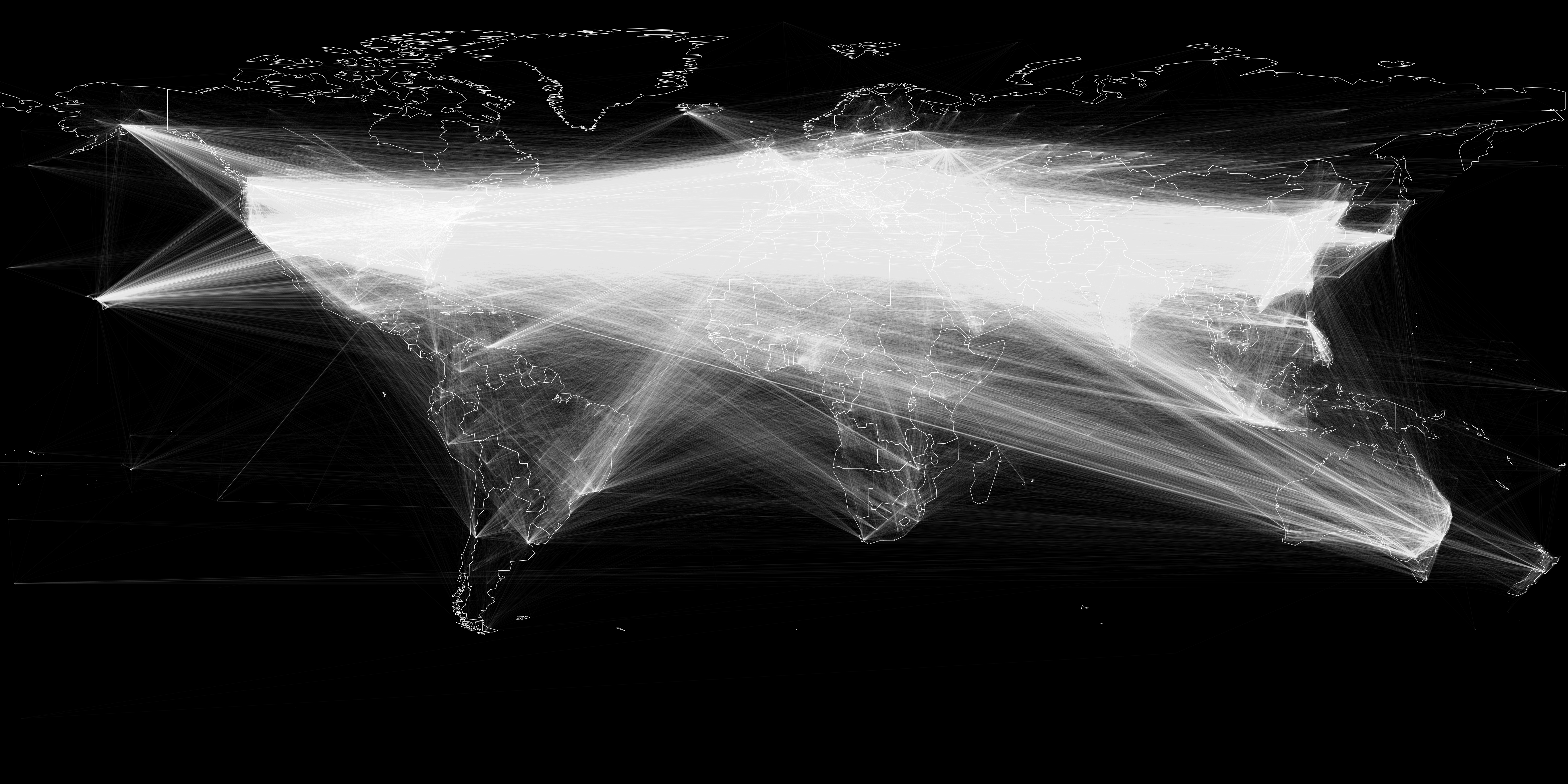
The map below repeats the analysis, but uses a cutoff of requiring that a pair of cities be mentioned together in at least 2,000 articles to yield a slightly less dense graph. Here the strongest links can be seen as a band that runs through the center of the world.

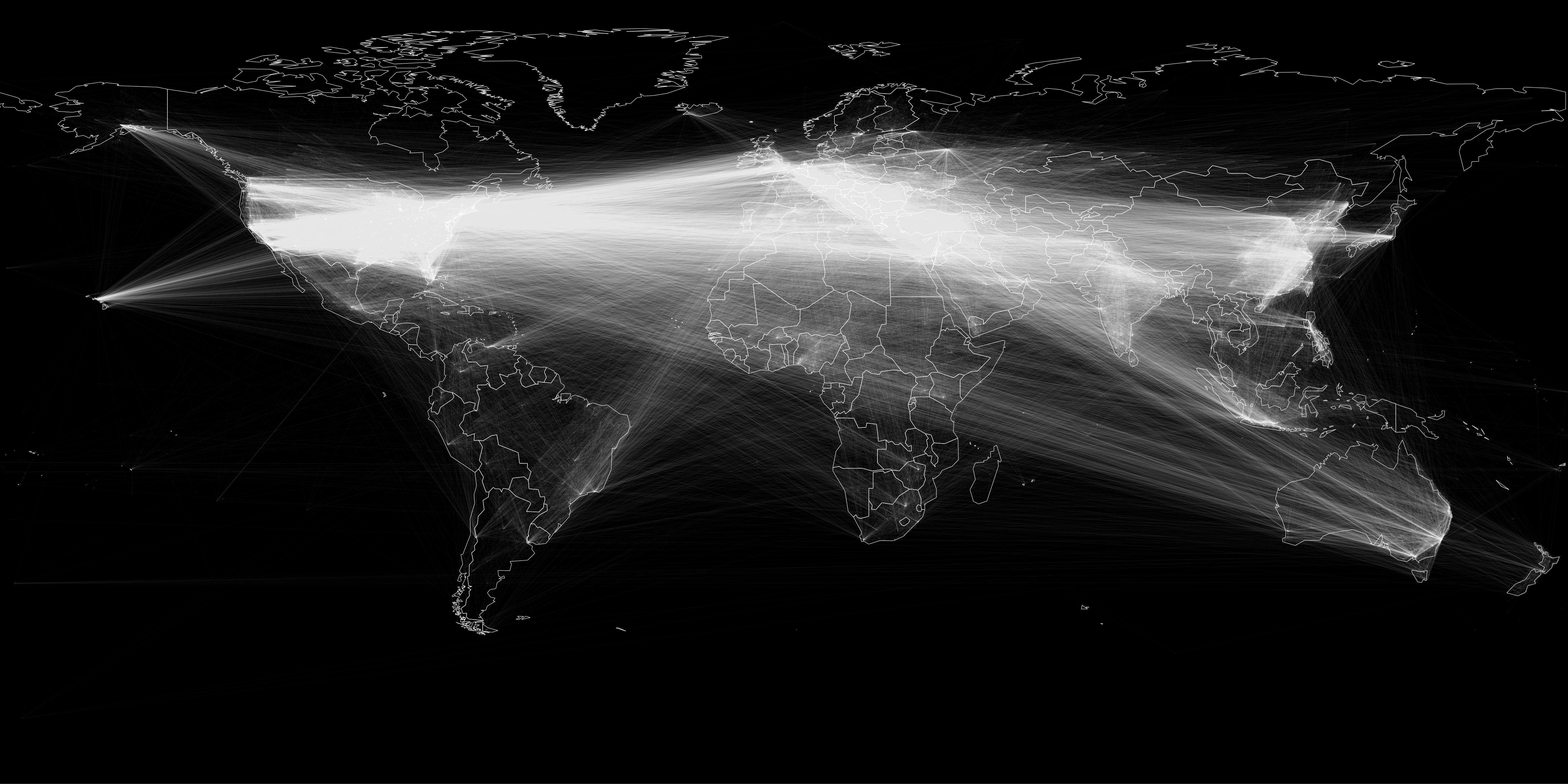
Increasing the threshold even further, the map below shows only the top 250,000 most-connected cities.

 

TECHNICAL DETAILS

To create the maps above, download the PNG basemaps from the original 2015 analysis and install GraphViz and ImageMagick. If necessary, adjust the default ImageMagick environmental configuration per the instructions from the 2018 analysis. Finally, use the updated "networkvisualizer.pl" Perl script that has an updated composite invocation that does a better job blending the network render with the basemap.

The graph construction SQL, courtesy of Felipe Hoffa, has been updated to Standard SQL and is seen below. Change the PARTITIONTIME parameters to adjust the specific time period examined by the analysis.

SELECT Source, Target, Count FROM (
SELECT a.coord Source, b.coord Target, COUNT(*) as Count
FROM (

(select GKGRECORDID, coord from (
WITH nested AS (
SELECT GKGRECORDID, SPLIT(V2Locations,';') locations FROM `gdelt-bq.gdeltv2.gkg_partitioned` WHERE _PARTITIONTIME >= "2015-01-01 00:00:00" AND _PARTITIONTIME <= "2015-12-31 23:59:59"
) select GKGRECORDID, CONCAT( CAST( ROUND(SAFE_CAST( IFNULL( REGEXP_EXTRACT(location,r'^[2-5]#.*?#.*?#.*?#.*?#(.*?)#') , '0') AS FLOAT64), 3) AS STRING), '#', CAST( ROUND(SAFE_CAST( IFNULL( REGEXP_EXTRACT(location,r'^[2-5]#.*?#.*?#.*?#.*?#.*?#(.*?)#') , '0') AS FLOAT64), 3) AS STRING) ) coord from nested, unnest(locations) location
) where coord != '0#0')

) a
JOIN (

(select GKGRECORDID, coord from (
WITH nested AS (
SELECT GKGRECORDID, SPLIT(V2Locations,';') locations FROM `gdelt-bq.gdeltv2.gkg_partitioned` WHERE _PARTITIONTIME >= "2015-01-01 00:00:00" AND _PARTITIONTIME <= "2015-12-31 23:59:59"
) select GKGRECORDID, CONCAT( CAST( ROUND(SAFE_CAST( IFNULL( REGEXP_EXTRACT(location,r'^[2-5]#.*?#.*?#.*?#.*?#(.*?)#') , '0') AS FLOAT64), 3) AS STRING), '#', CAST( ROUND(SAFE_CAST( IFNULL( REGEXP_EXTRACT(location,r'^[2-5]#.*?#.*?#.*?#.*?#.*?#(.*?)#') , '0') AS FLOAT64), 3) AS STRING) ) coord from nested, unnest(locations) location
) where coord != '0#0')

) b
ON a.GKGRECORDID=b.GKGRECORDID
WHERE a.coord<b.coord
GROUP BY 1,2
HAVING Count > 1000
ORDER BY 3 DESC
)