Powering the TV, TV AI and Visual Explorers is a petabyte-scale GCS archive consisting of hundreds of millions of discrete files, ranging from tens-of-gigabytes MPEG and MP4 files to small JSON, XML, SRT and other support files in a range of file formats. Historically we had no way of truly inventorying and understanding this vast archive sort of compiling lengthy archive-scale GCS inventories or using vast clusters of machines to mass-read key statistical files and render those results into final reports using bespoke tools. With the launch of GDELT 5.0, we now use GCP's Bigtable to construct a digital twin over our entire GCS archive, with all critical detail about each task (from ingest to processing via ASR, OCR, CV, GT and NLP GCP AI APIs to a range of other analytic and support tasks)  represented as a JSON blob. Unfortunately, as a no-SQL key-value store, Bigtable's massive scalability becomes problematic when we want to understand our vast archive at complete archive scale, running large-scale aggregation and other analytic tasks on top of it. Enter BigQuery's Bigtable connector. It turns out that BigQuery can actually be connected to Bigtable and bring to bear its full massive analytic capabilities to a Bigtable table just as it would any other BigQuery table and allow us to use ordinary SQL to perform all sorts of aggregations and analyses on our archive. What does this look like in practice?

In all, we performed a series of analyses using simple SQL on our digital twin covering 4.1M broadcasts totaling 10.9 billion seconds (182M minutes / 3M hours) of news programming totaling 1 quadrillion pixels analyzed by the Visual Explorer, leveraging BigQuery's JSON parsing and aggregation capabilities to chart various statistics and even deep-dive into a specific day to diagnose an anomaly. In all, these queries took just 6m22s to run @ 3.97GB processed, with a peak of 72,288 rows per second and 64MiB/s read throughput, peaking at just 3% additional CPU load on our Bigtable cluster.

The first step in connecting BigQuery to a Bigtable table is to create an external table connection. We do this by running this query in the BigQuery GCP web console. This tells BigQuery how to access our Bigtable table. Note that in this case both are in the same project. For use cases anticipating high analytic loads on their Bigtable tables that cannot tolerate additional load, simply add a second Bigtable cluster mirroring the first dedicated to BigQuery analytics and Bigtable will seamlessly mirror the data over.

CREATE EXTERNAL TABLE bigtableconnections.iatv_digtwin
OPTIONS (
  format = 'CLOUD_BIGTABLE',
  uris = ['https://googleapis.com/bigtable/projects/[YOURPROJECTID]/instances/[YOURBIGTABLEINSTANCE]/tables/iatv_digtwin'],
  bigtable_options =
    """
    {
      columnFamilies: [
        {
          "familyId": "cf",
          "type": "STRING",
          "encoding": "BINARY"
        }
      ],
      readRowkeyAsString: true
    }
    """
);

In our case, each broadcast is inserted into the digital twin with its date in YYYYMMDD as a prefix ala "20240818-theshowid", while each task output is stored in its own column as a JSON blob. In this case, we can perform a trivial query for all ingest records (stored in the "DOWN" column) that were successfully downloaded via:

SELECT rowkey, ( select array(select value from unnest(cell)) from unnest(cf.column) where name in ('DOWN') ) DOWN,
FROM `[YOURPROJECTID].bigtableconnections.digtwin` where rowkey like '20240818%' having DOWN like '%DOWNLOADED_SUCCESS%'

Of course, this isn't anything more powerful than what we can already do within Bigtable itself using its native capabilities. Here's where the magic begins. Let's leverage BigQuery's JSON parsing and aggregation capabilities to plot the total number of successfully downloaded broadcasts and their total airtime, as well as the total number of pixels analyzed by the Visual Explorer over time by day. We'll use JSON_EXTRACT_SCALAR() to extract the details we need from the DOWN JSON block and aggregate using a standard SQL statement:

SELECT DATE, COUNT(1) totShows, ROUND(SUM(sec)) totSec, ROUND(SUM(pixels)) totVEPixels from (
select substr(rowkey, 0, 8) as date,
  CAST(JSON_EXTRACT_SCALAR(DOWN, '$.durSec') AS FLOAT64) sec,
  (
    (CAST(JSON_EXTRACT_SCALAR(DOWN, '$.durSec') AS FLOAT64) / 4) * 
    CAST(JSON_EXTRACT_SCALAR(DOWN, '$.height') AS FLOAT64) * 
    CAST(JSON_EXTRACT_SCALAR(DOWN, '$.width') AS FLOAT64)
  ) AS pixels FROM (
  SELECT  
  rowkey, ( select array(select value from unnest(cell))[OFFSET(0)]  from unnest(cf.column) where name in ('DOWN') ) DOWN
  FROM `[YOURPROJECTID].bigtableconnections.iatv_digtwin` 
 ) WHERE DOWN like '%DOWNLOADED_SUCCESS%'
) group by date order by date

Let's plot the total number of successfully ingested shows by date. Here we can see a combination of the collection's actual structure (largely due to EPG data) and non-transient failures in ingesting videos. Using this graph we were able to immediately spot a number of date ranges to run advanced diagnostic systems to examine and understand to what degree there is a legitimate reduction of videos in that period vs an ingest system failure. Already we're getting some powerful results! In all, there were 4.1M news programs in the collection.

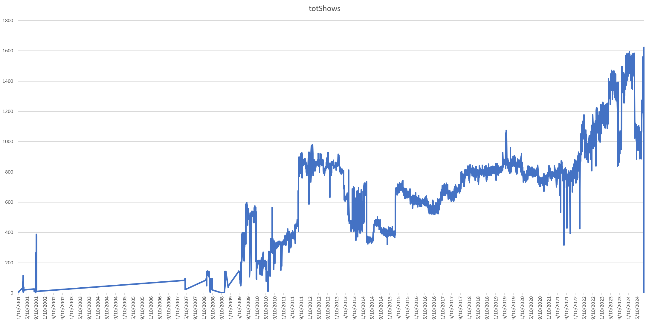
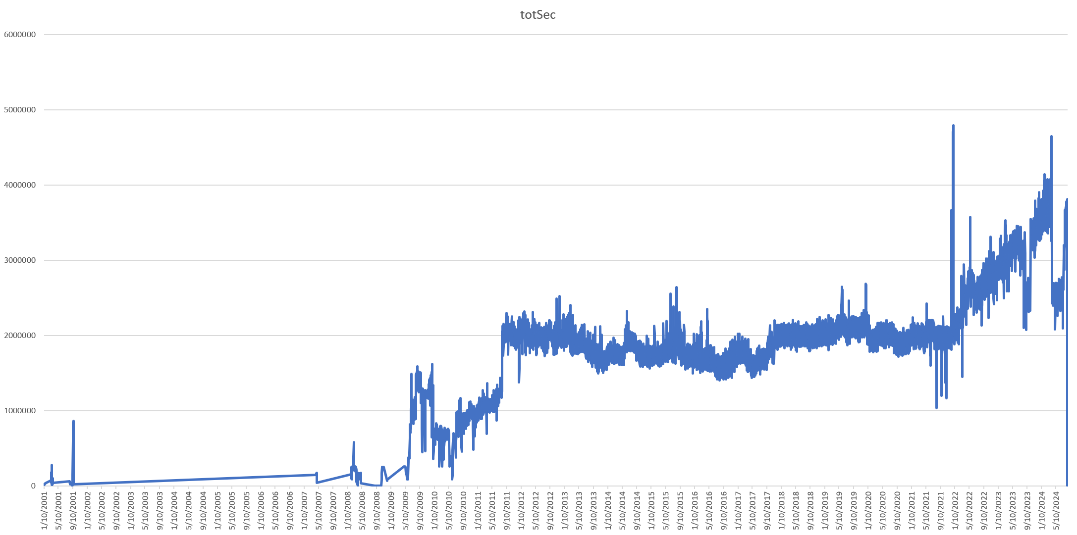
Interestingly, our diagnostic systems failed to pick up any major systematic ingest failures around those date ranges that would explain the sharp dips in the daily show count. What if we instead plot the daily seconds of news programming airtime in the archive? This graph looks very different and shows far more stability over time. This suggests that many of the trends above are due to shifts in EPG show cutting (whether airtime is grouped into fewer longer shows or more fine-grained shorter programs) rather than monitored airtime. In all, there are 10.9B seconds (182M minutes / 3M hours) of news programming airtime in the collection.

What about total pixels analyzed by the Visual Explorer? In all, there are just over 1.056 quadrillion pixels. However, there is a strange massive outlier on December 30, 2022. What might explain it?

Let's modify our query to return the complete inventory of shows from that day and sort by VE pixel count:

select rowkey,
JSON_EXTRACT_SCALAR(DOWN, '$.durSec') sec,
(
  (CAST(JSON_EXTRACT_SCALAR(DOWN, '$.durSec') AS FLOAT64) / 4) * 
  CAST(JSON_EXTRACT_SCALAR(DOWN, '$.height') AS FLOAT64) * 
  CAST(JSON_EXTRACT_SCALAR(DOWN, '$.width') AS FLOAT64)
) AS pixels,
DOWN FROM (
SELECT  
rowkey, ( select array(select value from unnest(cell))[OFFSET(0)]  from unnest(cf.column) where name in ('DOWN') ) DOWN
 FROM `[YOURPROJECTID].bigtableconnections.digtwin` where rowkey like '20211230%' 
) WHERE DOWN like '%DOWNLOADED_SUCCESS%' order by pixels desc

Immediately, the outlier becomes clear. A series of corrupt broadcasts that were not flagged as corrupt by the derivation process. One broadcast reports that it is 3.5 hours long when it actually represents only 30 minutes of programming, but most critically, its metadata reports that the video signal is 22,702 pixels wide by 12,768 pixels high – an impossibly high resolution for a channel that ordinarily broadcasts in standard HD.

Using a similar approach, we can run any kind of aggregation, analysis or filtering imaginable.