This is a guest post by Andrew Halterman.
Edit 17 Sept to reflect changes in dplyr‘s syntax
GDELT is an incredible resource for researchers and political scientists and has been getting increasing attention in popular publications. But weighing in at more than 60 GB, it’s too hefty for any kind of quick analysis in R, and is even cumbersome to subset in Python. The creators of GDELT suggest loading it into a SQL database, but this adds an extra layer of complexity for users, especially those (like me), who aren’t SQL experts. Enter Hadley Wickham’s dplyr, a faster version of plyr, built on the idea that “regardless of whether your data in an SQL database, a data frame or a data table, you should interact with it in the exactly the same way.” Meaning you tell dplyr what you want, and it handles the translation into SQL syntax.
I’ll explain how to go from a folder of csv‘s to dplyr speediness in three steps:
1. Creating the SQLite database.
2. Loading the GDELT data into the SQLite database.
3. Installing dplyr and running some basic operations
(If you haven’t already downloaded the GDELT dataset, do that first. John Beieler’s Python script makes the process painless.)
Creating the SQLite database (for neophytes)
For the purposes of this tutorial I’ll assume that you’re on a Mac, which comes with SQLite already installed. Things get a bit hairy later with compiling packages, so I have no idea to what extent YMMV on another OS.
To make sure everything’s working, go to your terminal and type
user$ sqlite3 test.db
It should tell you the version of SQLite you’re running (3.7.12 in my case) and give you asqlite3 prompt. You’ve created a database called test.db. To create a test table, type
sqplite> CREATE TABLE testtable(varchar, text)
This will create a table called testtable inside test.db, and the table will have a value column and a text column. This step isn’t important unless it doesn’t work. Type .quit and check your home folder, where you should see a test.db file. If it’s there, you can delete it. If it’s not, you’ll have to do some troubleshooting.
Loading the GDELT data into the database
We’ll create one database (gdelt.db) with two tables, GDELT_HISTORICAL and GDELT_DAILY. The reason for this is that GDELT_DAILY has an additional column listing the SOURCEURL, whichGDELT_HISTORICAL does not have.
In the terminal, create a new database called gdelt.db
user$ sqlite3 gdelt.db
From inside SQLite, create the table for historical GDELT files. (This SQL command is provided on the GDELT site)
CREATE TABLE GDELT_HISTORICAL (
 GLOBALEVENTID bigint(2) ,
 SQLDATE int(11) ,
 MonthYear char(6) ,
 Year char(4) ,
 FractionDate double ,
 Actor1Code char(3) ,
 Actor1Name char(255) ,
 Actor1CountryCode char(3) ,
 Actor1KnownGroupCode char(3) ,
 Actor1EthnicCode char(3) ,
 Actor1Religion1Code char(3) ,
 Actor1Religion2Code char(3) ,
 Actor1Type1Code char(3) ,
 Actor1Type2Code char(3) ,
 Actor1Type3Code char(3) ,
 Actor2Code char(3) ,
 Actor2Name char(255) ,
 Actor2CountryCode char(3) ,
 Actor2KnownGroupCode char(3) ,
 Actor2EthnicCode char(3) ,
 Actor2Religion1Code char(3) ,
 Actor2Religion2Code char(3) ,
 Actor2Type1Code char(3) ,
 Actor2Type2Code char(3) ,
 Actor2Type3Code char(3) ,
 IsRootEvent int(11) ,
 EventCode char(4) ,
 EventBaseCode char(4) ,
 EventRootCode char(4) ,
 QuadClass int(11) ,
 GoldsteinScale double ,
 NumMentions int(11) ,
 NumSources int(11) ,
 NumArticles int(11) ,
 AvgTone double ,
 Actor1Geo_Type int(11) ,
 Actor1Geo_FullName char(255) ,
 Actor1Geo_CountryCode char(2) ,
 Actor1Geo_ADM1Code char(4) ,
 Actor1Geo_Lat float ,
 Actor1Geo_Long float ,
 Actor1Geo_FeatureID int(11) ,
 Actor2Geo_Type int(11) ,
 Actor2Geo_FullName char(255) ,
 Actor2Geo_CountryCode char(2) ,
 Actor2Geo_ADM1Code char(4) ,
 Actor2Geo_Lat float ,
 Actor2Geo_Long float ,
 Actor2Geo_FeatureID int(11) ,
 ActionGeo_Type int(11) ,
 ActionGeo_FullName char(255) ,
 ActionGeo_CountryCode char(2) ,
 ActionGeo_ADM1Code char(4) ,
 ActionGeo_Lat float ,
 ActionGeo_Long float ,
 ActionGeo_FeatureID int(11) ,
 DATEADDED int(11)

);
Because GDELT files are tab-delimited, you need to tell SQLite to treat tabs as separators. From inside sqlite3 in the terminal, type
.separator t
After that, you can begin importing your pre-April 2013 GDELT files into the GDELT_HISTORICALtable using the form
.import /your_path_to_files/200601.csv GDELT_HISTORICAL
.import /your_path_to_files/200602.csv GDELT_HISTORICAL
.import /your_path_to_files/200603.csv GDELT_HISTORICAL
inserting the path to the GDELT files on your computer. You can copy-paste commands manually, or you can create a document with the list of all the file paths you’d like to import. Make you you include .separator t at the top of your file.
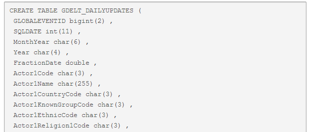
Now we do the same for the post-April daily updates. We create a second table insidegdelt.db.
CREATE TABLE GDELT_DAILYUPDATES (
 GLOBALEVENTID bigint(2) ,
 SQLDATE int(11) ,
 MonthYear char(6) ,
 Year char(4) ,
 FractionDate double ,
 Actor1Code char(3) ,
 Actor1Name char(255) ,
 Actor1CountryCode char(3) ,
 Actor1KnownGroupCode char(3) ,
 Actor1EthnicCode char(3) ,
 Actor1Religion1Code char(3) ,
 Actor1Religion2Code char(3) ,
 Actor1Type1Code char(3) ,
 Actor1Type2Code char(3) ,
 Actor1Type3Code char(3) ,
 Actor2Code char(3) ,
 Actor2Name char(255) ,
 Actor2CountryCode char(3) ,
 Actor2KnownGroupCode char(3) ,
 Actor2EthnicCode char(3) ,
 Actor2Religion1Code char(3) ,
 Actor2Religion2Code char(3) ,
 Actor2Type1Code char(3) ,
 Actor2Type2Code char(3) ,
 Actor2Type3Code char(3) ,
 IsRootEvent int(11) ,
 EventCode char(4) ,
 EventBaseCode char(4) ,
 EventRootCode char(4) ,
 QuadClass int(11) ,
 GoldsteinScale double ,
 NumMentions int(11) ,
 NumSources int(11) ,
 NumArticles int(11) ,
 AvgTone double ,
 Actor1Geo_Type int(11) ,
 Actor1Geo_FullName char(255) ,
 Actor1Geo_CountryCode char(2) ,
 Actor1Geo_ADM1Code char(4) ,
 Actor1Geo_Lat float ,
 Actor1Geo_Long float ,
 Actor1Geo_FeatureID int(11) ,
 Actor2Geo_Type int(11) ,
 Actor2Geo_FullName char(255) ,
 Actor2Geo_CountryCode char(2) ,
 Actor2Geo_ADM1Code char(4) ,
 Actor2Geo_Lat float ,
 Actor2Geo_Long float ,
 Actor2Geo_FeatureID int(11) ,
 ActionGeo_Type int(11) ,
 ActionGeo_FullName char(255) ,
 ActionGeo_CountryCode char(2) ,
 ActionGeo_ADM1Code char(4) ,
 ActionGeo_Lat float ,
 ActionGeo_Long float ,
 ActionGeo_FeatureID int(11) ,
 DATEADDED int(11) ,
 SOURCEURL char(255)
);
Loading the downloaded GDELT files into this table is the same as before, just with the table name changed to GDELT_DAILYUPDATES.
.import /your_path_to_files/20130401.export.csv GDELT_DAILYUPDATES
.import /your_path_to_files/20130402.export.csv GDELT_DAILYUPDATES
.import /your_path_to_files/20130403.export.csv GDELT_DAILYUPDATES
etc.
When you’re done loading all of the files into their corresponding tables, you’re done with the SQL part (until tomorrow’s GDELT update) and we can move on to dplyr.
Installing and using dplyr
Big caveat Okay, actually there’s a Step 1.9 for some of you. dplyr requires a compiler (make) that was taken out in OS 10.8. To install make if you’re on Snow Leopard and don’t have it already, download and install Xcode from the App Store (I know, sorry) and go to Xcode > Preference > Downloads and insall the Command Line Tools.
dplyr is still under development on GitHub and is not yet part of CRAN. To download dplyrfrom GitHub, use Hadley Wickham’s devtools.
library(devtools)
install_github("assertthat")
install_github("dplyr")
install.packages("RSQLite")
install.packages("RSQLite.extfuns")
Hadley recommends that dplyr and plyr not be loaded simultaneously.
Now we load the packages:
library(dplyr)
library(RSQLite)
library(RSQLite.extfuns)
Once all of the packages are set up, we can tell dplyr how to access our two tables, providing the path to the database and then the table name. Replace my path with yours, of course.
****This is where the syntax is different****
daily.db <- source_sqlite("/Volumes/ahalt/gdelt.db", "GDELT_DAILYUPDATES")
hist.db <- source_sqlite("/Volumes/ahalt/gdelt.db", "GDELT_HISTORICAL")gdelt.db <- src_sqlite("/Volumnes/ahalt/gdelt.db") daily.db <- tbl(gdelt.db, "GDELT_DAILYUPDATES")hist.db <- tbl(gdelt.db, "GDELT_HISTORICAL")
dplyr give you five basic operations for working with your remote data. filter will return rows based on criteria you determine, select will return the columns you specify, arrange will re-order your rows, mutate will add columns, and summarise will perform by-group operations on your data. dplyr also offers a do command which applies any arbitrary function to your data, which is very useful for say, applying a linear model to each group in your data. We’re primarily interested in the first two and summarise. For a full list of commands and to check for syntax updates (which might be coming soon), visit Hadley Wickham’s GitHub page.
Let’s say we’re interested in where events have occured in Syria since. We can filter the database by ActionGeo_CountryCode like this (remember to use two letter FIPS country codes, not three letter ISO)
syria <- filter(daily.db, ActionGeo_CountryCode == "SY")
and then select only the rows we’re interested in.
syria <- select(syria, ActionGeo_Long, ActionGeo_Lat, ActionGeo_FullName)
If we wanted to export this data directly to a data frame to view or work with, we could export it with:
syria.df <- as.data.frame(syria, n=-1)
The n=-1 prints all the rows rather than the default first 100,000.
We’re going to press on, though, and look at what dplyr can do in the way of aggregating. Perhaps we’re interested in how many events happen at each location. We can tell dplyr to group by any number of variables.
syria <- group_by(syria, ActionGeo_Lat, ActionGeo_Long, ActionGeo_FullName)
Up to this point, the operations should have been essentially instant. This next operation, usingsummarise to sum events by ActionGeo_FullName will require a few minutes since it’s the first command to actually execute the query.
syria.count <- summarise(syria, count = n())
syria.count <- as.data.frame(syria.count)
This takes me 80 seconds on a 2009 MacBook Pro with the SQLite database on an external hard drive. It’s a bit faster on an Air reading off the SSD.
Typing
syria.count[order(-syria.count$count),]
shows us what we might expect, namely that the top three most common place names in Syria are “Syria”, “Damascus”, and “Aleppo” and they have an overwhelming 124,522 out of 161,218 total events since April. (See my post with David Masad for more on GDELT’s geocoding).
To map:
library(ggplot2)
library(ggmap)
syria.map <- qmap(location = "syria", maptype = "terrain", color = "bw", zoom = 7)
syria.map + geom_point(data = syria.count, aes(x = ActionGeo_Long, y = ActionGeo_Lat,
    size = log(count)), color = "red", alpha = 0.6)

dplyr output map of Syria
There’s much more to be done with the do function and some more speed tests, but that’s for another post. Leave a comment with any questions you have or send me a message on Twitter @ahalterman.