Embeddings are designed to look beyond the words on a page to the semantic concepts they represent, allowing a search for "dogs" to match articles that mention "golden retrievers", a search for "doctor" to match "medical professional", a "road" to match a "street" and so on. There are myriad commercial and open embedding models available today, so as part of our generative AI series, today we'll showcase a Colab template you can use to compare different models in your own content domain and use it to explore the impact of capitalization, spacing and knowledge cutoffs in embedding models.
We will include templates for four models from the Universal Sentence Encoder (USE) family, including the English-only USEv4, the larger English-only USEv5-Large, the 16-language USEv3-Multilingual and the larger 16-language USEv3-Multilingual-Large models. The multilingual models support 16 languages (Arabic, Chinese-simplified, Chinese-traditional, English, French, German, Italian, Japanese, Korean, Dutch, Polish, Portuguese, Spanish, Thai, Turkish, Russian). We'll also compare with the 100-language LaBSEv2 model that is optimized for translation-pair scoring. Finally, we'll test with the Vertex AI Embeddings for Text API.
Here we will compare six sentences that test capitalization ("Monkeypox" vs "monkeypox"), spacing ("monkeypox" vs "monkey pox") and knowledge cutoffs (the introduction of "mpox" as an alternative preferred replacement for Monkeypox in November 2022):
sentences = [
    "Mpox cases continue to climb",
    "mpox cases continue to climb",
    "Monkey pox cases continue to climb",
    "monkey pox cases continue to climb",
    "Monkeypox cases continue to climb",
    "monkeypox cases continue to climb",
]
Those interested in the code can skip to the bottom of the this post for the complete notebook code and step-by-step instructions to replicate the analyses here for your own set of sentences.
Overall findings:
- Capitalization Sensitivity. Most of the models are highly sensitive to capitalization, meaning that editorial differences in news articles and/or the informal capitalization of social media can result in highly dissimilar embeddings.
- Internal Spacing. Some terms, especially emergent ones, can lack standardized rules on internal spacing, such as "monkeypox" versus "monkey pox." All of the embedding models differentiate these different forms, making it more difficult to look across spacing differences.
- Knowledge Cutoffs. Embedding models represent a snapshot in time of language use. In theory, their use of "word parts" or "tokens" in place of whole words is supposed to allow them to better handle OOV (out of vocabulary) terms (words they have not seen before), but the results here show that, as expected, if a model has never seen a word before, it cannot easily group it with its synonyms, just as a human seeing "mpox" for the first time would not likely immediately recognize it as a replacement term for "monkeypox." Some models grouped "mpox" and "monkeypox" more closely than others, while others more strongly stratified them. Since none of the models have knowledge cutoffs after the introduction of "mpox" this offers a real-world example of how model aging can negatively impact the ability of embedding models to support semantic search for breaking terminology. Indeed, the world knowledge encoded by Gecko is now nearly two years old, meaning all of the myriad words introduced over that time are not accurately captured in its semantic graph. Importantly, this means that in fast-moving disciplines with constantly expanding and evolving terminology, models will have to be constantly updated. At the same time, each model update will require recomputing the entire database of previously-computed embeddings due to the updated model. An archive of trillions of social media post embeddings will have to be regenerated from scratch every time the embedding model is updated with new terminology – meaning that realistically most models will not be frequently updated. For longer passages of text, the surrounding context should be sufficient to at least group them into somewhat similar bins, but when encoding short social media posts and user search queries, this will be a significant problem.
Vertex Embedding API
Let's start with the Vertex AI Embeddings for Text API. This is a small LLM called "embedding-gecko-001" that is part of the PaLM 2 family. The knowledge cutoff for the family is mid-2021, meaning that since "Mpox" was introduced in November 2022, the model won't know that "mpox" is the same as "Monkeypox".
You can see the pairwise similarity scores below, showing that Gecko is highly sensitive to all three difference classes (capitalization, spacing and knowledge cutoff):
[[0.99999952 0.976166 0.87537304 0.87547783 0.91140729 0.89990498]
[0.976166 0.9999997 0.86688576 0.86786797 0.89675627 0.88878286]
[0.87537304 0.86688576 0.99999979 0.96388279 0.9728849 0.9606419 ]
[0.87547783 0.86786797 0.96388279 0.99999976 0.95423151 0.98140475]
[0.91140729 0.89675627 0.9728849 0.95423151 0.99999991 0.97556736]
[0.89990498 0.88878286 0.9606419 0.98140475 0.97556736 0.99999966]]
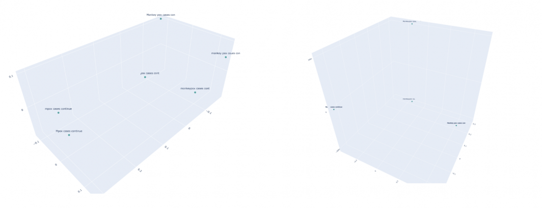
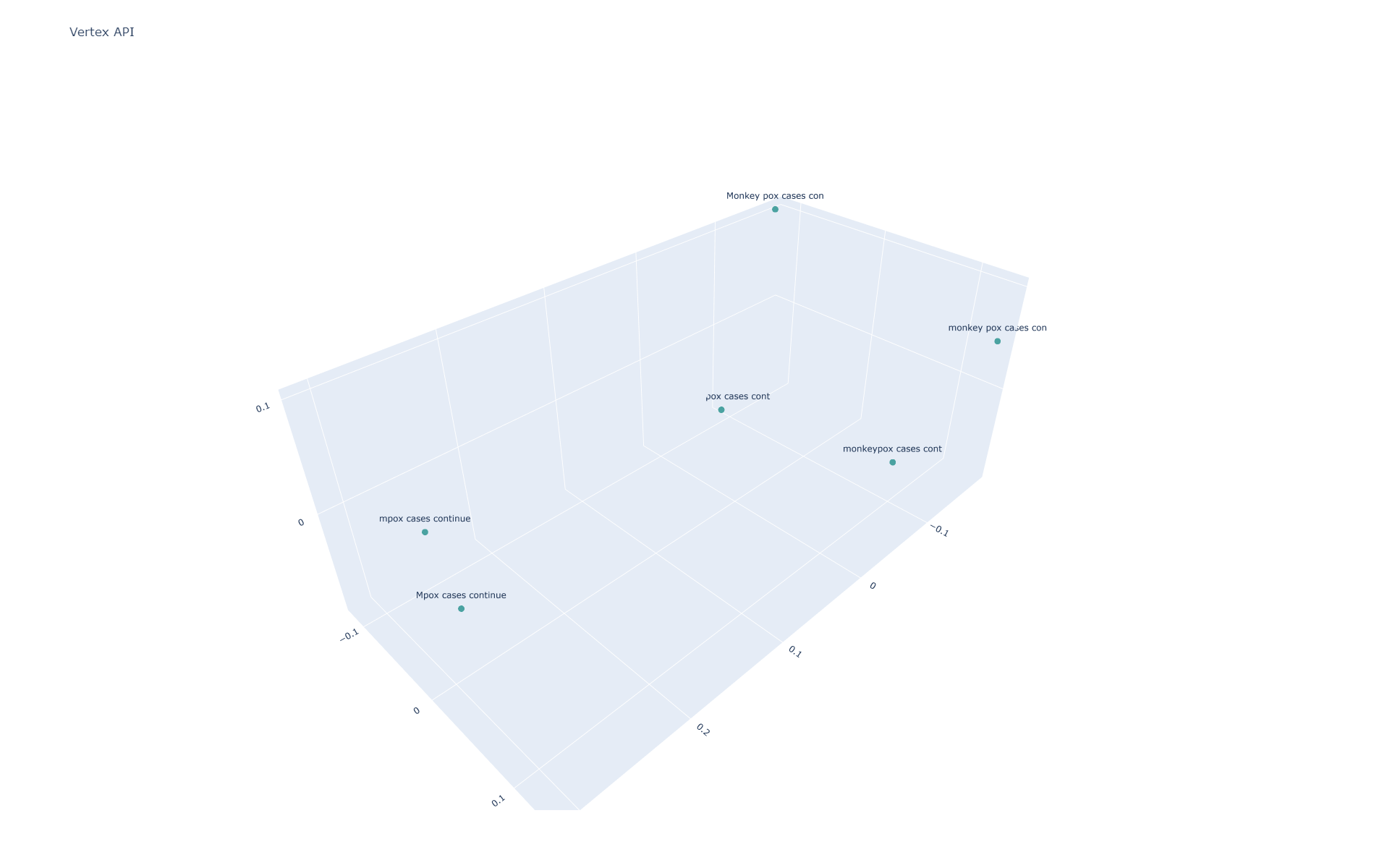
Using PCA to project into 3 dimensions and visualizing (the labels are truncated to the first 10 characters to fit onto the graph), we can see that, other than mpox and monkeypox being separated than the others, all six sentences are fairly spaced apart
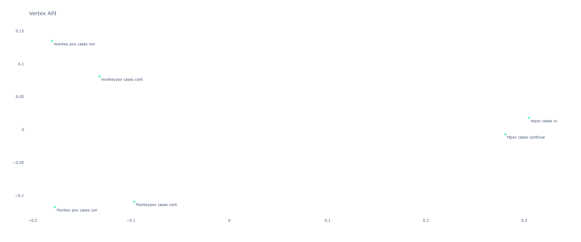
If we project into two dimensions we can see this trend even more clearly:
Universal Sentence Encoder
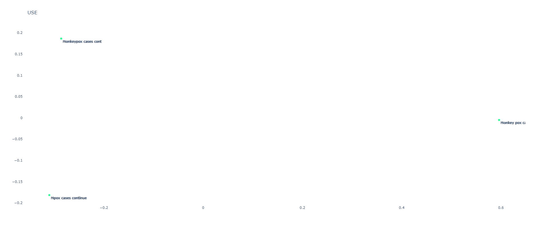
The base USE model is insensitive to capitalization, but sensitive to the other two classes:
[[1.0000002 1.0000002 0.5736684 0.5736684 0.93195546 0.93195546]
[1.0000002 1.0000002 0.5736684 0.5736684 0.93195546 0.93195546]
[0.5736684 0.5736684 0.9999999 0.9999999 0.59238577 0.59238577]
[0.5736684 0.5736684 0.9999999 0.9999999 0.59238577 0.59238577]
[0.93195546 0.93195546 0.59238577 0.59238577 1. 1. ]
[0.93195546 0.93195546 0.59238577 0.59238577 1. 1. ]]
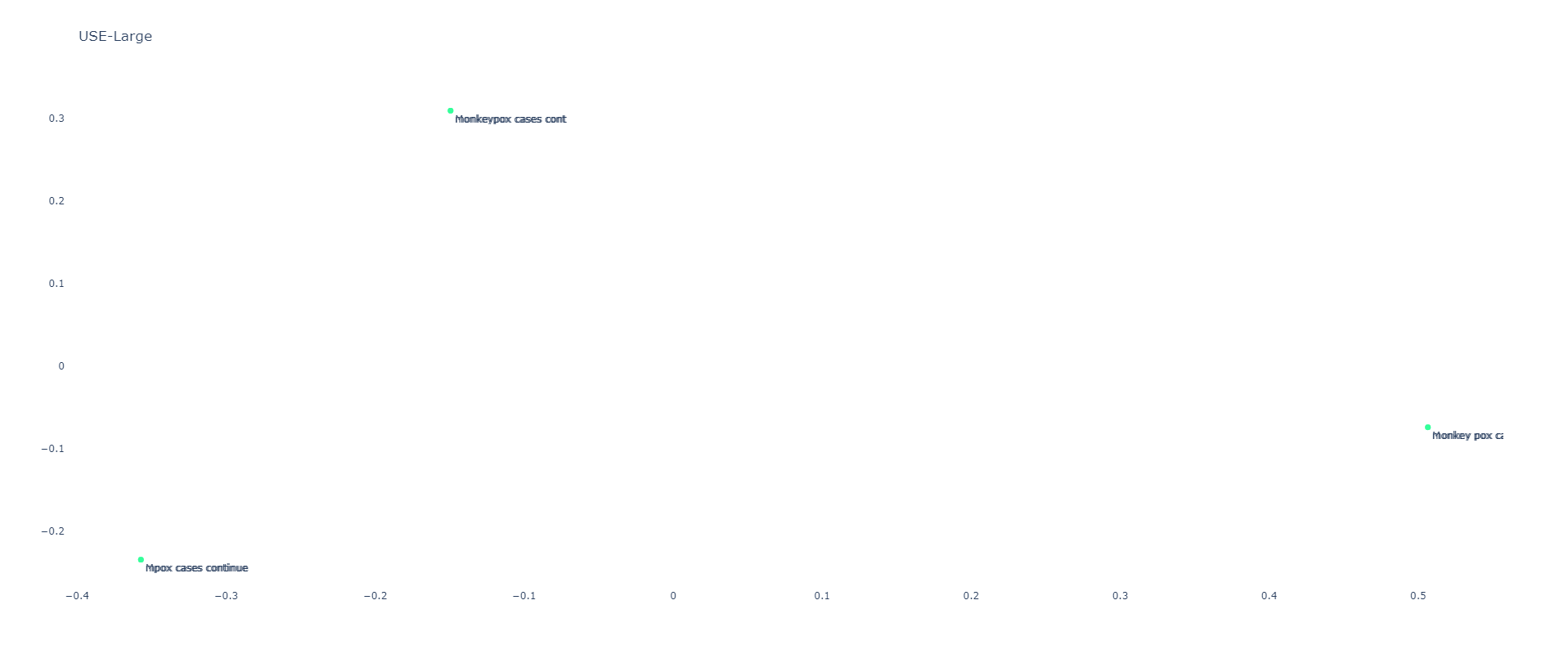
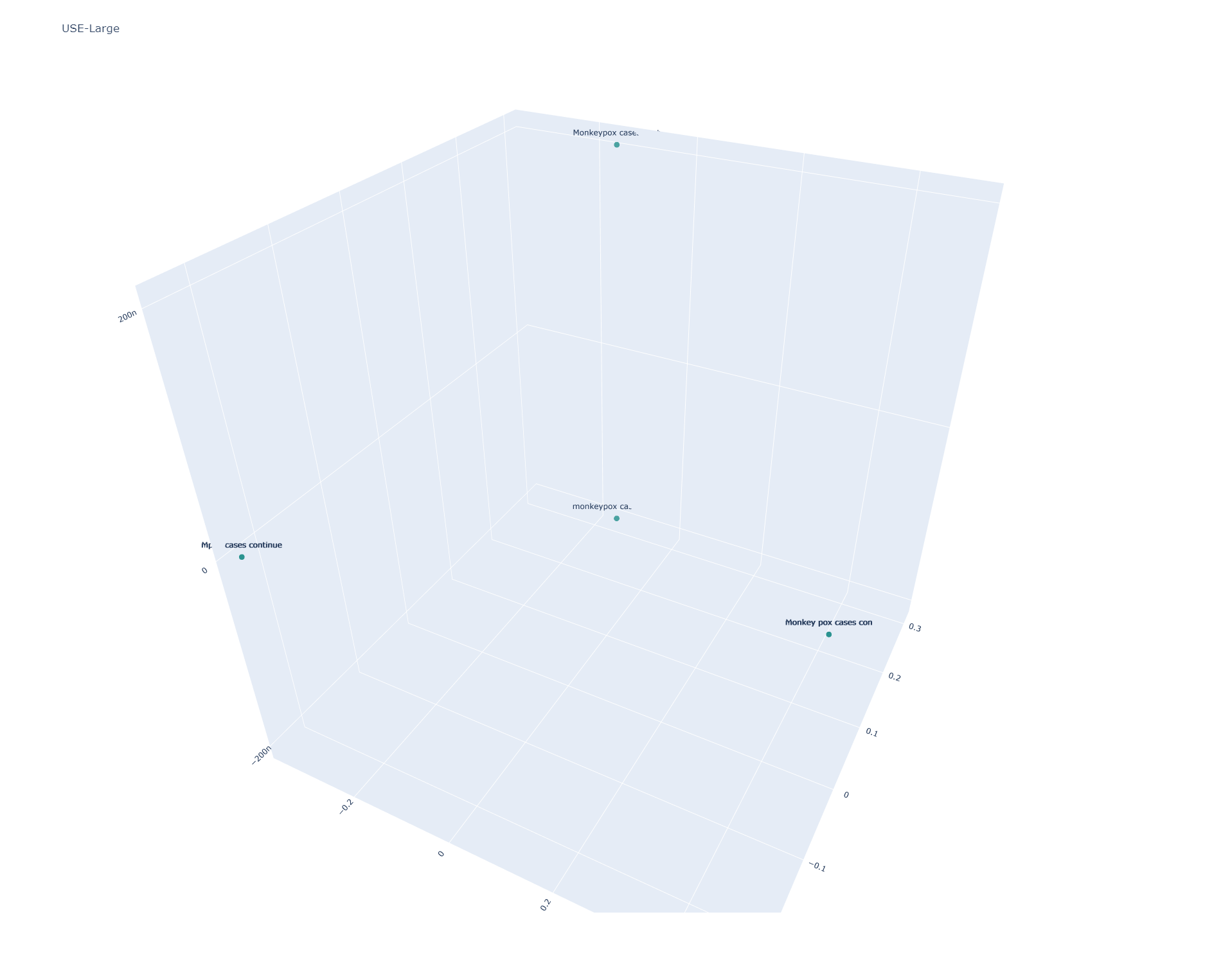
Universal Sentence Encoder Large
USE Large yields nearly identical results to USE:
[[1.0000002 1.0000002 0.6141466 0.6141466 0.8302376 0.8302375 ]
[1.0000002 1.0000002 0.6141466 0.6141466 0.8302376 0.8302375 ]
[0.6141466 0.6141466 1.0000002 1.0000002 0.7112366 0.7112365 ]
[0.6141466 0.6141466 1.0000002 1.0000002 0.7112366 0.7112365 ]
[0.8302376 0.8302376 0.7112366 0.7112366 0.99999976 0.99999976]
[0.8302375 0.8302375 0.7112365 0.7112365 0.99999976 0.99999976]]
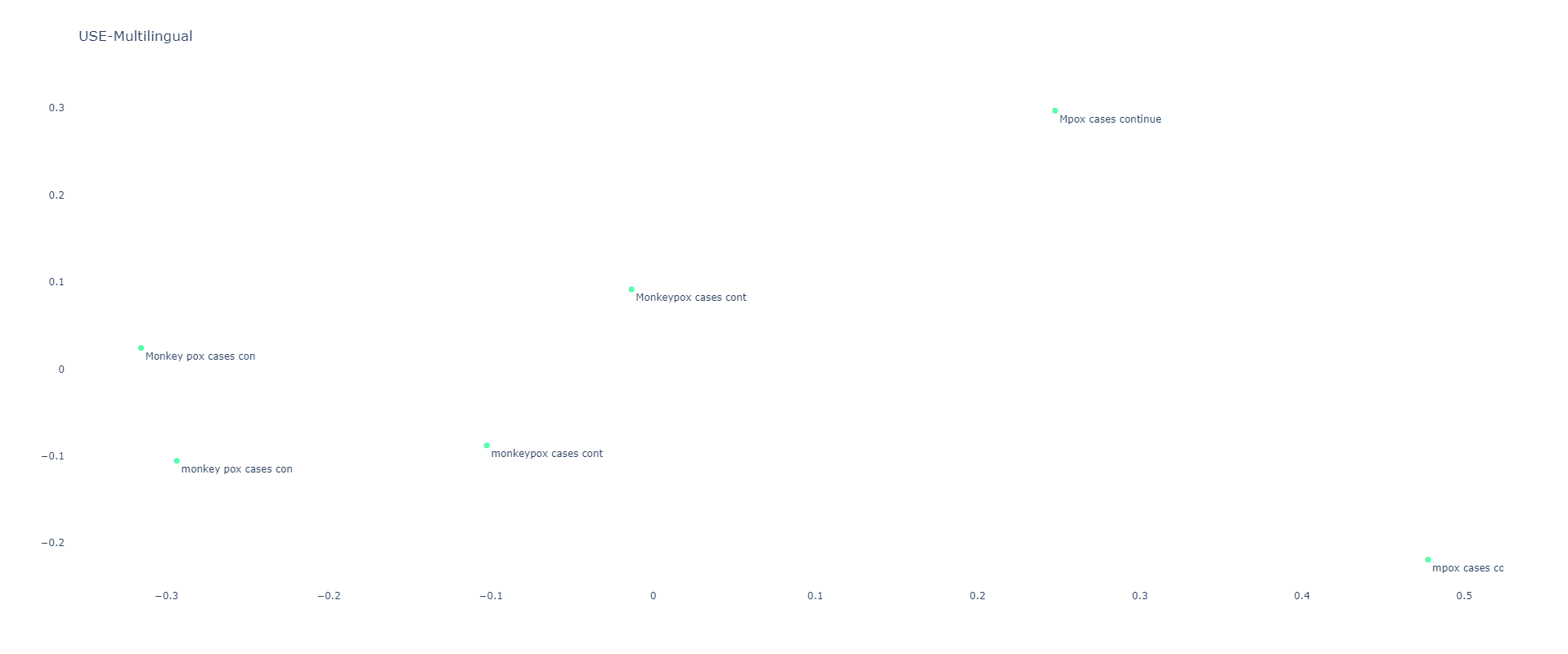
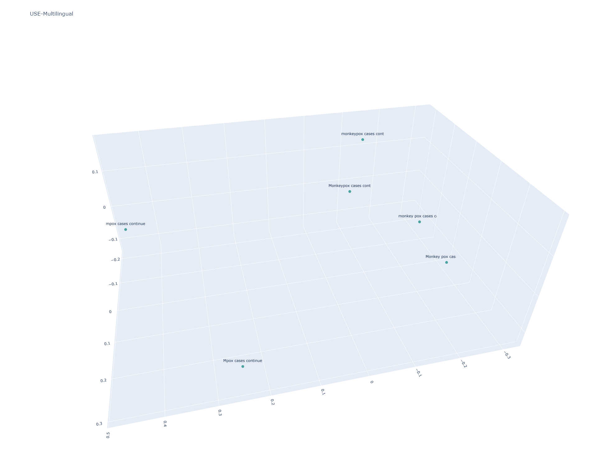
Universal Sentence Encoder Multilingual
USE Multilingual is case sensitive, resulting in all six sentences being scattered:
[[1. 0.8307743 0.77761847 0.76908386 0.88787407 0.83321553]
[0.8307743 1. 0.6490631 0.6823242 0.79888666 0.7786906 ]
[0.77761847 0.6490631 1.0000002 0.95740235 0.90316945 0.8950101 ]
[0.76908386 0.6823242 0.95740235 1.0000001 0.8784237 0.9369095 ]
[0.88787407 0.79888666 0.90316945 0.8784237 1. 0.9373039 ]
[0.83321553 0.7786906 0.8950101 0.9369095 0.9373039 1.0000001 ]]
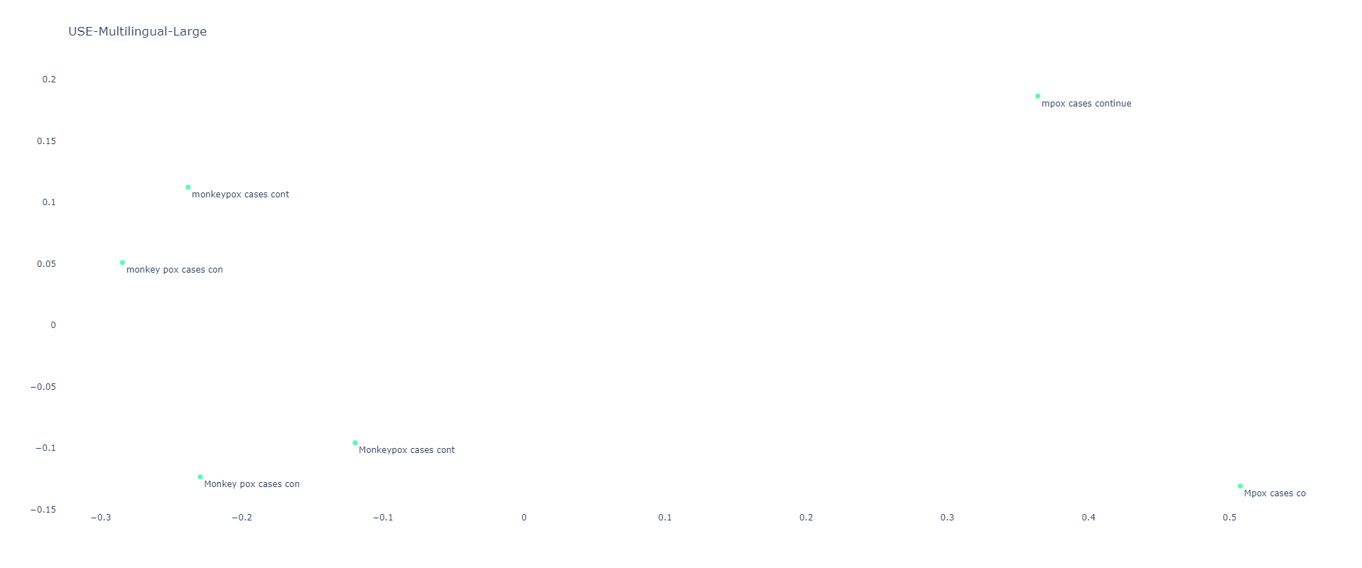
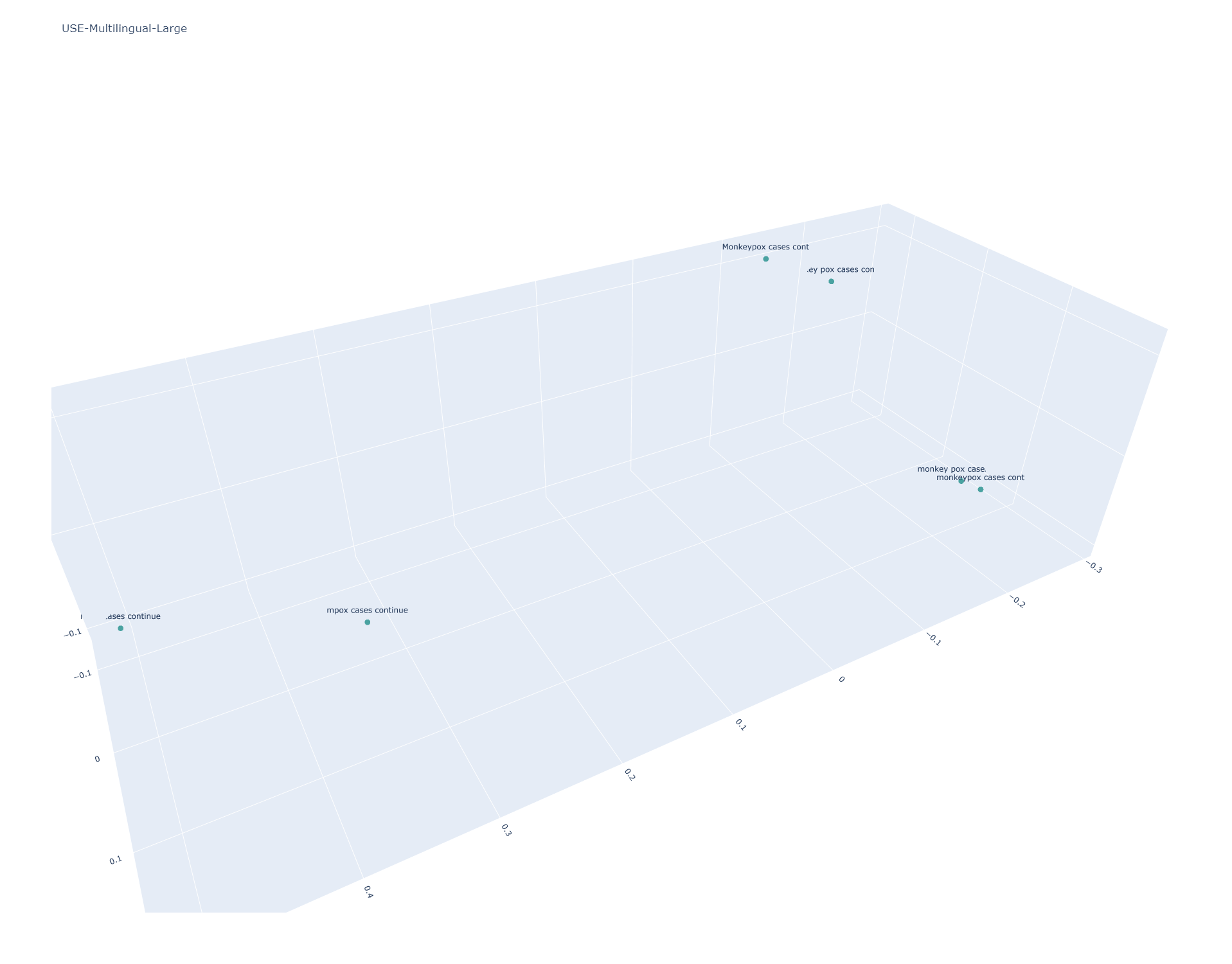
Universal Sentence Encoder Multilingual Large
Here the results are similar to the main USE Multilingual model, but the Large edition results in stronger stratification of "mpox" from "monkeypox". Given the knowledge cutoffs of these models, this is a more desirable effect within the bounds of the model's knowledge, but for actual real-world applications in 2023 is undesirable.
[[0.99999994 0.91871804 0.71093345 0.66713125 0.7764429 0.6895789 ]
[0.91871804 1.0000002 0.773957 0.75960815 0.8370214 0.79734755]
[0.71093345 0.773957 1.0000001 0.9673796 0.9797696 0.9535649 ]
[0.66713125 0.75960815 0.9673796 1.0000001 0.9432931 0.9868417 ]
[0.7764429 0.8370214 0.9797696 0.9432931 1.0000002 0.95375013]
[0.6895789 0.79734755 0.9535649 0.9868417 0.95375013 0.99999976]]
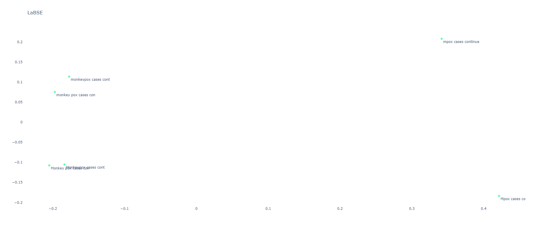
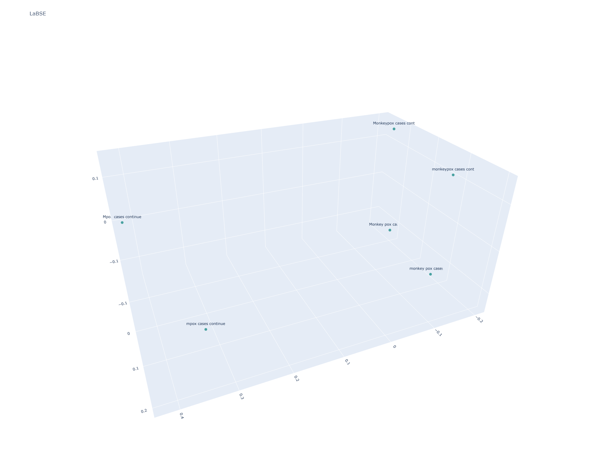
LaBSE
LaBSE stratifies the sentences similarly to USE Multilingual Large:
[[0.9999999 0.90897745 0.78381854 0.7656153 0.79353976 0.7685686 ]
[0.90897745 1.0000002 0.7942246 0.8262198 0.80083156 0.83916414]
[0.78381854 0.7942246 1.0000004 0.97264147 0.96323764 0.933204 ]
[0.7656153 0.8262198 0.97264147 1. 0.9336194 0.96427447]
[0.79353976 0.80083156 0.96323764 0.9336194 1. 0.96434927]
[0.7685686 0.83916414 0.933204 0.96427447 0.96434927 0.9999998 ]]
Notebook Template
To create these graphs, first create a new Colab notebook and then paste the following code into it.
First, we'll paste the sentences to examine:
sentences = [
    "Mpox cases continue to climb",
    "mpox cases continue to climb",
    "Monkey pox cases continue to climb",
    "monkey pox cases continue to climb",
    "Monkeypox cases continue to climb",
    "monkeypox cases continue to climb",
]
Then we'll create our 3D visualization function. This also uses DBSCAN to cluster the embeddings and colors the points by cluster. In the case of the sentences above, there was insufficient clustering, so they were all labeled as outliers.
from sklearn.decomposition import PCA
import plotly.graph_objs as graph
import numpy as np
from sklearn.cluster import DBSCAN
from sklearn.neighbors import NearestNeighbors

def embedPCAVisual3D(embeds, graphtitle):
    #collapse to 3D via PCA...
    pca = PCA(n_components=3)
    embeds_pca = pca.fit_transform(embeds)
    #print(embeds_pca.tolist())

    #compute the optimal epsilon value for DBSCAN
    #compute the k-distance graph
    neigh = NearestNeighbors(n_neighbors=2) #adjust to the minimum number of points required for a cluster
    neigh.fit(embeds)
    distances, _ = neigh.kneighbors(embeds)
    k_distances = np.sort(distances[:, -1])
    #compute the knee point
    differences = np.diff(k_distances)
    knee_index = np.argmax(differences) + 1
    #epsilon is the distance at knee point
    epsilon = k_distances[knee_index]
    print("Optimal Epsilon: ", epsilon)

    #cluster via DBSCAN
    cluster = DBSCAN(metric="euclidean", n_jobs=-1, eps=epsilon)
    cluster.fit(embeds)
    print(cluster.labels_)

    trace = graph.Scatter3d(
        x=embeds_pca[:, 0],
        y=embeds_pca[:, 1],
        z=embeds_pca[:, 2],
        marker=dict(
            size=5,
            #color=np.arange(len(embeds_pca)), #color randomly
            color=cluster.labels_, #color via DBSCAN clusters
            colorscale='Viridis',
            opacity=0.8
        ),
        text=[sentence[:20] for sentence in sentences],
        hoverinfo='text',
        mode='markers+text'
    )

    layout = graph.Layout(
        title=graphtitle,
        scene=dict(
            xaxis=dict(title=''),
            yaxis=dict(title=''),
            zaxis=dict(title=''),
        ),
        height=1200
    )

    fig = graph.Figure(data=[trace], layout=layout)
    fig.update_layout(hovermode='closest', hoverlabel=dict(bgcolor="white", font_size=12))
    fig.show()

    #override the max height of the cell to fully display the graph
    from IPython.display import Javascript
    display(Javascript('''google.colab.output.setIframeHeight(0, true, {maxHeight: 1200})'''))
And our 2D visualizer:
from sklearn.decomposition import PCA
import plotly.graph_objs as graph
import numpy as np
from sklearn.cluster import DBSCAN
from sklearn.neighbors import NearestNeighbors

def embedPCAVisual2D(embeds, graphtitle):
    #collapse to 3D via PCA...
    pca = PCA(n_components=2)
    embeds_pca = pca.fit_transform(embeds)
    #print(embeds_pca.tolist())

    #compute the optimal epsilon value for DBSCAN
    #compute the k-distance graph
    neigh = NearestNeighbors(n_neighbors=2) #adjust to the minimum number of points required for a cluster
    neigh.fit(embeds)
    distances, _ = neigh.kneighbors(embeds)
    k_distances = np.sort(distances[:, -1])
    #compute the knee point
    differences = np.diff(k_distances)
    knee_index = np.argmax(differences) + 1
    #epsilon is the distance at knee point
    epsilon = k_distances[knee_index]
    print("Optimal Epsilon: ", epsilon)

    #cluster via DBSCAN
    cluster = DBSCAN(metric="euclidean", n_jobs=-1, eps=epsilon)
    cluster.fit(embeds)
    print(cluster.labels_)

    trace = graph.Scatter(
        x=embeds_pca[:, 0],
        y=embeds_pca[:, 1],
        marker=dict(
            size=7,
            #color=np.arange(len(embeds_pca)), #color randomly
            color=cluster.labels_, #color via DBSCAN clusters
            colorscale='Rainbow',
            opacity=0.8
        ),
        text=[sentence[:20] for sentence in sentences],
        hoverinfo='text',
        mode='markers+text',
        textposition='bottom right'
    )

    layout = graph.Layout(
        title=graphtitle,
        scene=dict(
            xaxis=dict(title=''),
            yaxis=dict(title=''),
        ),
        height=800,
        plot_bgcolor='rgba(0,0,0,0)'
    )

    fig = graph.Figure(data=[trace], layout=layout)
    fig.update_layout(hovermode='closest', hoverlabel=dict(bgcolor="white", font_size=12))
    #fig.update_xaxes(showline=True, linewidth=2, linecolor='lightgrey', gridcolor='lightgrey')
    #fig.update_yaxes(showline=True, linewidth=2, linecolor='lightgrey', gridcolor='lightgrey')
    fig.show()

    #override the max height of the cell to fully display the graph
    from IPython.display import Javascript
    display(Javascript('''google.colab.output.setIframeHeight(0, true, {maxHeight: 1000})'''))
To test with the Vertex Text Embeddings API, add this code to your notebook. Note that you'll need to enable the Vertex API in your GCP project. To call the Vertex API, this code requires you to grant your notebook access to your GCP credentials. If you don't wish to do so, you can skip this block and proceed to the next section. You'll also need to change the "[YOURPROJECTIDHERE]" in the code below to your GCP Project ID:
from google.colab import auth
auth.authenticate_user()
import numpy as np
import json

#compute the embeddings
embeds = []
for i in range(len(sentences)):
    !rm cmd.json
    !rm results.json
    print("Embedding: ", sentences[i])
    data = {"instances": [ {"content": sentences[i]} ]}
    with open("cmd.json", "w") as file: json.dump(data, file)
    cmd = 'curl -s -X POST -H "Authorization: Bearer $(gcloud auth print-access-token)" -H "Content-Type: application/json; charset=utf-8" -d @cmd.json "https://us-central1-aiplatform.googleapis.com/v1/projects/[YOURPROJECTIDHERE]/locations/us-central1/publishers/google/models/textembedding-gecko:predict" > results.json'
    !{cmd}
    with open('results.json', 'r') as f: data = json.load(f)
    print(data)
    embeds.append(np.array(data['predictions'][0]['embeddings']['values']))

#prevent NP from line-wrapping when printing the arrays below
np.set_printoptions(linewidth=500)

#compare them
simmatrix = np.inner(embeds, embeds)
print(simmatrix)

#visualize them
embedPCAVisual2D(embeds, "Vertex API")
embedPCAVisual3D(embeds, "Vertex API")
To test with the open offline models, this cell will install and load all five models:
!pip3 install tensorflow_text>=2.0.0rc0

import tensorflow_hub as hub
import numpy as np
import tensorflow_text

embed_use = hub.load("https://tfhub.dev/google/universal-sentence-encoder/4")
embed_use_large = hub.load("https://tfhub.dev/google/universal-sentence-encoder-large/5")
embed_use_multilingual = hub.load("https://tfhub.dev/google/universal-sentence-encoder-multilingual/3")
embed_use_multilingual_large = hub.load("https://tfhub.dev/google/universal-sentence-encoder-multilingual-large/3")

!pip install -U sentence-transformers
from sentence_transformers import SentenceTransformer
import numpy as np
labse = SentenceTransformer('sentence-transformers/LaBSE')
And then this will actually run them across all of the sentences:
#prevent NP from line-wrapping when printing the arrays below
np.set_printoptions(linewidth=500)

#USE
print("\nUSE")
%time results = embed_use(sentences)
simmatrix = np.inner(results, results)
print(simmatrix)
embedPCAVisual2D(results, "USE")
embedPCAVisual3D(results, "USE")

#USE-LARGE
print("\nUSE-LARGE")
%time results = embed_use_large(sentences)
simmatrix = np.inner(results, results)
print(simmatrix)
embedPCAVisual2D(results, "USE-Large")
embedPCAVisual3D(results, "USE-Large")

#USE-MULTILINGUAL
print("\nUSE-MULTILINGUAL")
%time results = embed_use_multilingual(sentences)
simmatrix = np.inner(results, results)
print(simmatrix)
embedPCAVisual2D(results, "USE-Multilingual")
embedPCAVisual3D(results, "USE-Multilingual")

#USE-MULTILINGUAL-LARGE
print("\nUSE-MULTILINGUAL-LARGE")
%time results = embed_use_multilingual_large(sentences)
simmatrix = np.inner(results, results)
print(simmatrix)
embedPCAVisual2D(results, "USE-Multilingual-Large")
embedPCAVisual3D(results, "USE-Multilingual-Large")

#LABSE
print("\nLABSE")
%time results = labse.encode(sentences)
simmatrix = np.inner(results, results)
print(simmatrix)
embedPCAVisual2D(results, "LaBSE")
embedPCAVisual3D(results, "LaBSE")
That's all there is to it! You can use this template to visualize the results for any set of sentences simply by replacing the sentence array at the beginning and rerunning the notebook!