
Last month we visualized the network of who appeared alongside whom in an episode of Russian TV news' "60 Minutes" using facial clustering. What would it look like to scale that up to an entire year of 60 Minutes episodes, spanning 342 broadcasts totaling 50,467 minutes of airtime, scanning more than 757,000 "video ngram" images to extract 774,615 human faces representing 4,972 distinct people and combine them into a massive graph of who appeared together alongside whom – yielding a massive graph of the world of 60 Minutes, all in the space of just a few hours?
Skip to the bottom of this post if you aren't interested in the technical aspects and just want to see the final graphs.
The entire analysis here was performed on a 64-core N1 GCE VM with 400GB RAM, using 200GB as a RAM disk. Everything below was performed in a subdirectory of /dev/shm/ to minimize IO latency.
First we'll install a couple of base dependencies:
apt-get -y install parallel
apt-get -y install jq
apt-get -y install wget
apt-get -y install zip
Then, we'll download all of the Visual Explorer 4-second visual ngrams for all episodes of 60 Minutes (since EPG data for Russia 1 begins May 19, 2022, the query below will only return shows from that date onward).
We'll begin by compiling a list of the IDs of all 60 Minutes broadcasts:
start=20220101; end=20230318; while [[ ! $start > $end ]]; do echo $start; start=$(date -d "$start + 1 day" "+%Y%m%d"); done > DATES
mkdir JSON
time cat DATES | parallel --eta 'wget -q https://storage.googleapis.com/data.gdeltproject.org/gdeltv3/iatv/visualexplorer/RUSSIA1.{}.inventory.json -P ./JSON/'
rm IDS.tmp; find ./JSON/ -depth -name '*.json' | parallel --eta 'cat {} | jq -r .shows[].id >> IDS.tmp'
grep '60_minut' IDS.tmp | sort > IDS
This yields a list of 342 broadcasts. Then we'll download the image ZIP files and unpack them (we highly recommend performing this in a RAM disk due to the number of small files involved):
mkdir IMAGES
time cat IDS | parallel --eta 'wget -q https://storage.googleapis.com/data.gdeltproject.org/gdeltv3/iatv/visualexplorer/{}.zip -P ./IMAGES/'
time find ./IMAGES/ -depth -name '*.zip' | parallel --eta 'unzip -n -q -d ./IMAGES/ {} && rm {}'
time find ./IMAGES/ -depth -name "*.jpg" | wc -l
This yields 757,559 total images. Now we're going to download a Python script and associated tooling that will extract all of the faces from each image and compute the embeddings for each.
First, we install the dependencies:
apt-get -y install build-essential
brew install cmake
pip3 install face_recognition
pip3 install imutils
pip3 install argparse
pip3 install scikit-learn
Now we're going to extract all of the faces and encode them as 128-dimension embeddings and store as a pickle. We use the Histogram of Oriented Gradients (HOG) detection method because we are running on a CPU-only system. While the CNN model would likely yield better results, this allows us to run without a GPU, though in practice during spot checks we did not identify any obvious failed facial extractions.
First we download the encoding script:
wget https://raw.githubusercontent.com/kunalagarwal101/Face-Clustering/master/encode_faces.py
The encoding script above processes a directory of images in serial, so we will parallelize it by running one copy of the script on each directory in parallel. On a 64-core system this takes around 4 hours to extract and encode all of the faces seen across all 757,000 images:
mkdir ENCODINGS
time find ./IMAGES/ -type d -name 'RUSSIA*' | parallel --eta 'python3 encode_faces.py --dataset {} --encodings ./ENCODINGS/{/}.encodings.pickle --detection_method "hog"'&
The script scans each image in the given directory in sequence, extracts all human faces, and computes a 128-dimension embedding for each. When it completes, it writes a pickle file containing the final results.
This means we will have one pickle file per broadcast, totaling 342 pickle files that collectively encode 774,615 faces. To cluster the complete dataset, we'll need to merge all of the pickle files together. Each of the pickles is a simple array, so we just need to load each pickle and merge all of their arrays together.
Save the following script as "mergeencodings.py":
import os
import pickle

dir='ENCODINGS/'
merged = []
for filename in os.listdir(dir):
    if filename.endswith('.pickle'):
        print(filename)
        data = pickle.loads(open(dir+filename, "rb").read())
        merged.extend(data)

print("Total entries: {}...".format(len(merged)))
print("Writing merge file...")
file = open("./MERGED.pickle","wb")
pickle.dump(merged, file)
file.close()
Then run it as:
time python3 ./mergeencodings.py
In less than 9 seconds it will take all 342 pickle files and merge them together. The final pickle file is an array of 774,615 embeddings.
Now it is time to cluster all of those embeddings to group them by face. Save the following script as "cluster_all.py":
from sklearn.cluster import DBSCAN
import pickle
import numpy as np
import json

print("[INFO] loading encodings...")
data = pickle.loads(open("./MERGED.pickle", "rb").read())
data = np.array(data)
encodings = [d["encoding"] for d in data]

print("[INFO] clustering...")
clt = DBSCAN(metric="euclidean", n_jobs=-1, eps=0.4)
clt.fit(encodings)

labelIDs = np.unique(clt.labels_)
numUniqueFaces = len(np.where(labelIDs > -1)[0])
print("[INFO] # unique faces: {}".format(numUniqueFaces))

file = open("./DATABASE.json","w")
for i in range(0,len(clt.labels_)):
    print(json.dumps({"faceid": int(clt.labels_[i]), "image": data[i]["imagePath"], "box": data[i]["loc"], "encoding": data[i]["encoding"].tolist() }), file=file)
file.close()
And run it as:
time python3 ./cluster_all.py
On our 64-core VM it takes just 5m11s to run, yielding 4,972 distinct faces. You can adjust the eps value above to cluster faces more or less aggressively. Smaller values yield tighter clusters at the risk of incorrectly splitting an accurate grouping of faces into different people, while larger values will group multiple people incorrectly into a single person. In practice we've found a value of 0.4 to provide the most accurate clustering performance on Russian television news. Given the speed of the clustering process, you can easily explore different values and spot check the results to see which works best for a given application.
The clustering script above outputs a massive JSON-NL database containing every single extracted human face (774,615 records in all), its identified cluster, the path to the original image, the bounding box to use to extract it and its embedding, one per row.
You can see a sample entry below (this has been reformatted to make it more readable – in the actual file the entire record appears on a single line):
{
"faceid": -1,
"image": "./IMAGES/RUSSIA1_20230317_143000_60_minut/RUSSIA1_20230317_143000_60_minut-000001.jpg",
"box": [126, 703, 216, 613],
"encoding": [-0.0772986114025116, 0.06904534995555878, 0.12260625511407852, 0.07705958187580109, -0.12215105444192886,
 0.025747139006853104, -0.08783647418022156, -0.06360627710819244, 0.04049253091216087, -0.07749307155609131,
 0.2278400957584381, -0.033374298363924026, -0.24538330733776093, -0.07759930193424225, -0.02369013801217079,
 0.08189386129379272, -0.12964583933353424, -0.14702628552913666, -0.08374384790658951, -0.041040580719709396,
 0.05492480844259262, 0.11911934614181519, 0.05884547159075737, -0.03724893555045128, -0.13534149527549744,
 -0.3687266707420349, -0.03602997213602066, -0.10086500644683838, 0.12097285687923431, -0.0757226049900055,
 -0.030660443007946014, 0.02202298864722252, -0.13137179613113403, -0.026274804025888443, 0.04703182354569435,
 0.14102499186992645, -0.08576402068138123, -0.014238985255360603, 0.21881458163261414, 0.009365606121718884,
 -0.2273736298084259, -0.012513515539467335, 0.03334633260965347, 0.2673637270927429, 0.19366204738616943,
 0.07736664265394211, 0.04852158948779106, -0.01713128201663494, 0.07608118653297424, -0.30479419231414795,
 0.1698392927646637, 0.14989283680915833, 0.15746620297431946, 0.08323390781879425, 0.14135198295116425,
 -0.22792449593544006, -0.04927489161491394, 0.18495257198810577, -0.13127687573432922, 0.15326769649982452,
 0.06208003684878349, -0.09212884306907654, 0.04295201227068901, -0.015411472879350185, 0.2069588005542755,
 0.05423096567392349, -0.09762626141309738, -0.155641108751297, 0.20565371215343475, -0.1631849706172943,
 -0.07215613126754761, 0.1885523498058319, -0.05560119077563286, -0.1361183375120163, -0.2565898597240448,
 0.03935761749744415, 0.4497328996658325, 0.08644187450408936, -0.16985149681568146, -0.02549273706972599,
 0.015545286238193512, -0.05014156922698021, 0.06695189327001572, 0.11815610527992249, -0.028687622398138046,
 -0.02950340509414673, -0.1398799866437912, -0.03280247747898102, 0.1637628674507141, 0.001592753455042839,
 -0.04253312572836876, 0.22626419365406036, 0.019924357533454895, 0.05580771341919899, 0.10259910672903061,
 0.05254768580198288, -0.08181627839803696, -0.0033469325862824917, -0.08030882477760315, -0.023593958467245102,
 0.007859259843826294, -0.12469752132892609, -0.014781113713979721, 0.07277587801218033, -0.07292212545871735,
 0.17672452330589294, -0.07415906339883804, 0.04843538627028465, 0.01942340098321438, -0.03560560196638107,
 -0.05275237560272217, 0.012793932110071182, 0.19044440984725952, -0.3313567042350769, 0.1819138526916504,
 0.14857400953769684, 0.02728659100830555, 0.16187886893749237, 0.07468220591545105, 0.08180717378854752,
 0.04954831302165985, -0.04781661927700043, -0.24659480154514313, -0.10279341787099838, -0.03762281686067581,
 -0.10649019479751587, -0.02194802463054657, 0.09079930931329727]
}
To extract the actual face image itself, combine the bounding box and image filename fields. The "box" dimensions are: top, right, bottom, left. Thus, in Perl you can combine as:
$coords = ($ref->{'box'}[1] - $ref->{'box'}[3]) . 'x' . ($ref->{'box'}[2] - $ref->{'box'}[0]) . '+' . $ref->{'box'}[3] . '+' . $ref->{'box'}[0];
print OUT $ref->{'image'} . "\t$extract\t$ref->{'faceid'}.$LINEID\n";
And then pass to ImageMagick to extract via:
mkdir IMAGENODES
time cat IMAGES.TXT | parallel --colsep "\t" --eta 'convert {1} -extract {2} ./IMAGENODES/{3}.jpg'
One challenge is that when looking across 774,615 faces, how does one pick the single "best" image to represent each person when displaying in a graph? Selecting the face with the largest bounding box or largest JPEG filesize will favor larger images or those with more detail, but those are not necessarily the best image. A larger image could actually reflect a case where the face extractor struggled to properly segment the face and combined it with too much background image, while a larger JPEG filesize could reflect a stylized image that has been heavily filtered.
Instead, a better approach would be to average or find the median of all of the embeddings (perhaps after removing outliers) for a given face to compute the most central representation of the face and then compute the distance of all examples of that face from that average embedding to find the "best" representation of the face. We leave that exercise for a future exploration.
You can download the complete database:
- FACEEMBED-60MINUTES-20220519-20230318.json.gz (900MB compressed / 2GB uncompressed)
Let's form this into a co-occurrence graph. Save the following into "makegephi_json.pl":
#!/usr/bin/perl

use JSON::XS;

#parse the database and build into a pre-graph...
open(FILE, $ARGV[0]);
while(<FILE>) {
    my $ref; eval { $ref = decode_json($_); }; if (!defined($ref)) { next; };
    if ($ref->{'faceid'} == -1) { next; }; #skip unassigneds...

    #and assign the face to this frame...
    ($show, $frame) = $ref->{'image'}=~/.*\/(.*?)\-(\d\d\d\d\d\d)\.jpg/;
    $FRAME_FACES{$show}{$frame}{$ref->{'faceid'}} = 1;

}
close(FILE);

#iterate by show and build our real graph...
foreach $show (keys %FRAME_FACES) {
    #loop over each frame in this show that had faces...
    foreach $frame (keys %{$FRAME_FACES{$show}}) {
	my @arr_thisfaceids = (sort keys %{$FRAME_FACES{$show}{$frame}});
	my @arr_lastfaceids = (sort keys %{$FRAME_FACES{$show}{$frame-1}});

	for($i=0;$i<scalar(@arr_thisfaceids);$i++) {
	    for($j=$i+1;$j<scalar(@arr_thisfaceids);$j++) { $EDGES{"$arr_thisfaceids[$i],$arr_thisfaceids[$j]"}+=2; } #this frame...
	    for($j=$i+1;$j<scalar(@arr_lastfaceids);$j++) { if ($arr_thisfaceids[$i] != $arr_thisfaceids[$j]) { $EDGES{"$arr_thisfaceids[$i],$arr_thisfaceids[$j]"}++; }; } #prev frame...
	}

    }
}

#sort the edges by strength and construct a graph of the top X stongest edges...
open(OUT, ">./EDGES.csv");
print OUT "Source,Target,Type,Weight,CocurFrames\n"; $WROTE = 0; $MAX = 0;
foreach $pair (sort {$EDGES{$b} <=> $EDGES{$a}} keys %EDGES) {
    if ($WROTE++ > 1000) { last; };
    if ($MAX == 0) { $MAX = $EDGES{$pair}; };
    $weight = sprintf("%0.4f", $EDGES{$pair} / $MAX);
    print OUT "$pair,\"Undirected\",$weight,$EDGES{$pair}\n";
    ($node1, $node2) = split/,/, $pair; $NODES{$node1} = 1; $NODES{$node2} = 1;
}
close(OUT);

#and output the final nodes graph...
open(OUT, ">./NODES.csv");
print OUT "Id,Label\n";
foreach $node (keys %NODES) {
    print OUT "$node,$node\n";
}
close(OUT);
And run via:
time ./makegephi_json.pl DATABASE.json
This will take around one minute and will connect all faces appearing in each frame and with all faces from the preceding frame (to connect across the back-and-forth camera shots common to Russian TV news). It will then sort them by strength and output the top 1,000 strongest connections as NODES.csv and EDGES.csv, ready to be imported directly into Gephi.
Load the graph into Gephi and use PageRank to size the nodes and modularity to color them by community finding (clustering), with Force Atlas 2 as the layout algorithm. Visualizing the final graph yields the following:
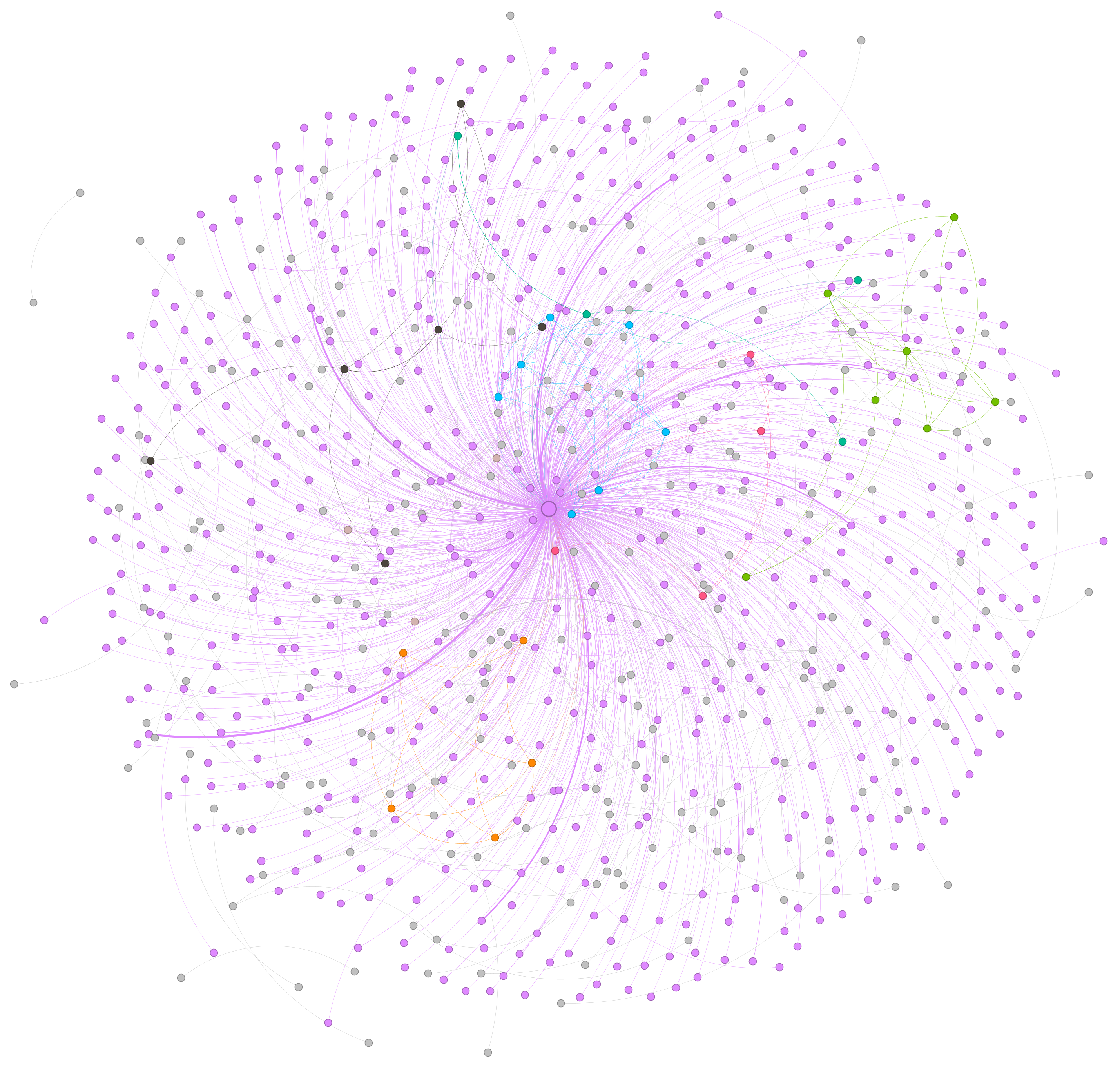
Immediately clear is that the entire world of 60 Minutes revolves around a single person: host Olga Skabeyeva. Interestingly, despite a few people having slightly stronger connections to her, there is no central cluster of a "central cast of characters" in the show – it revolves around Olga and Olga alone.
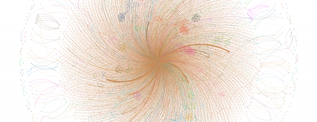
What if we expand the threshold in the script above from 1,000 to 10,000 and switch to OpenOrd to yield better clustering on this particular graph? In this particular network there are only 5,955 edges in total, counting even a single isolated co-occurrence over the entire year, capturing again just how much the show revolves around Olga, rather than myriad miniature clusters centering on various stories.
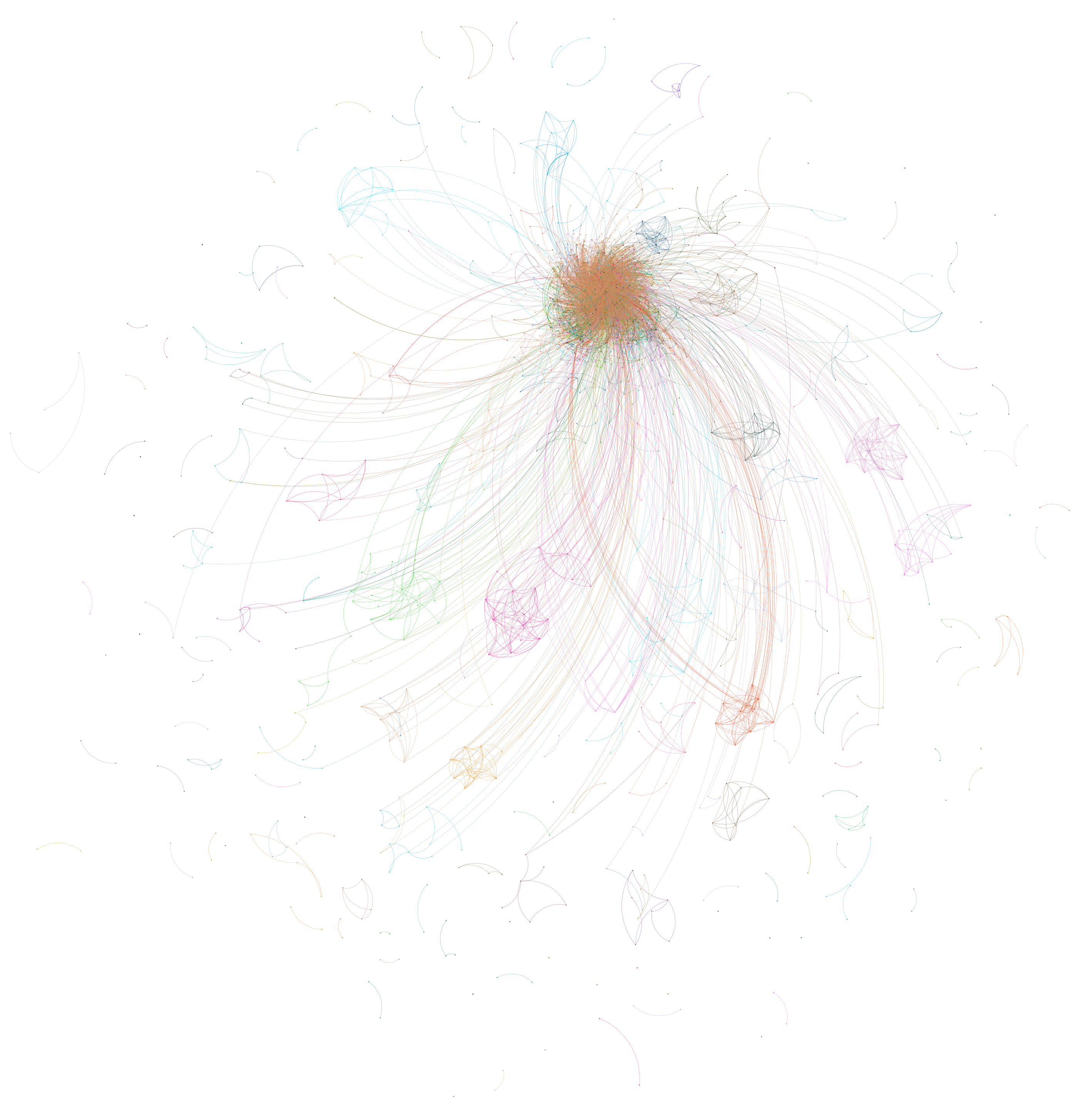
The central cluster above is hard to discern, so we'll use a different layout algorithm (Fruchterman Reingold) that gives us better separation by more evenly distributing the nodes. This offers perhaps the best visualization of a year of 60 Minutes episodes, showing Olga at the center with the entire world revolving around her. A few principles like her husband Yevgeny Popov are seen to be heavily connected to her, but they are merely radials from her, rather than forming a central nexus, reflecting that the camera, after shifting to them, shifts back to her to give her the last word before moving on to the next speaker.
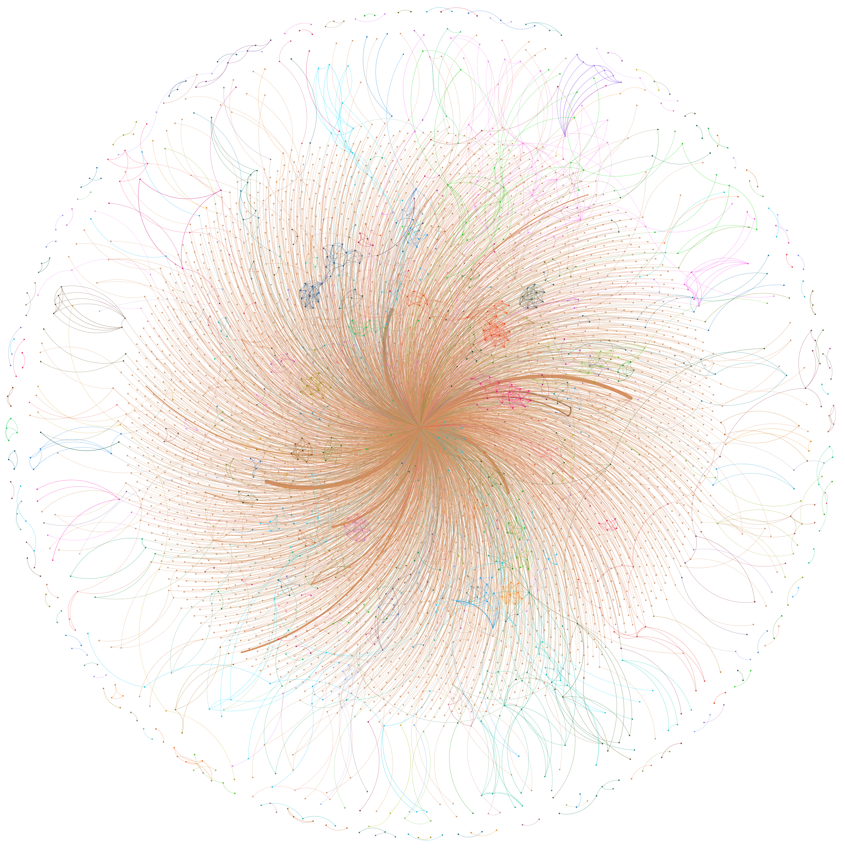
In a single graph we have the narrative speaker landscape of 60 Minutes, with Olga at its center, capturing who has appeared alongside of whom in a year of 60 Minutes. Most powerfully of all, this enormous analysis takes just a few hours on a single CPU-only VM, placing such immense longitudinal analyses within reach for any large television news series.